Introduction

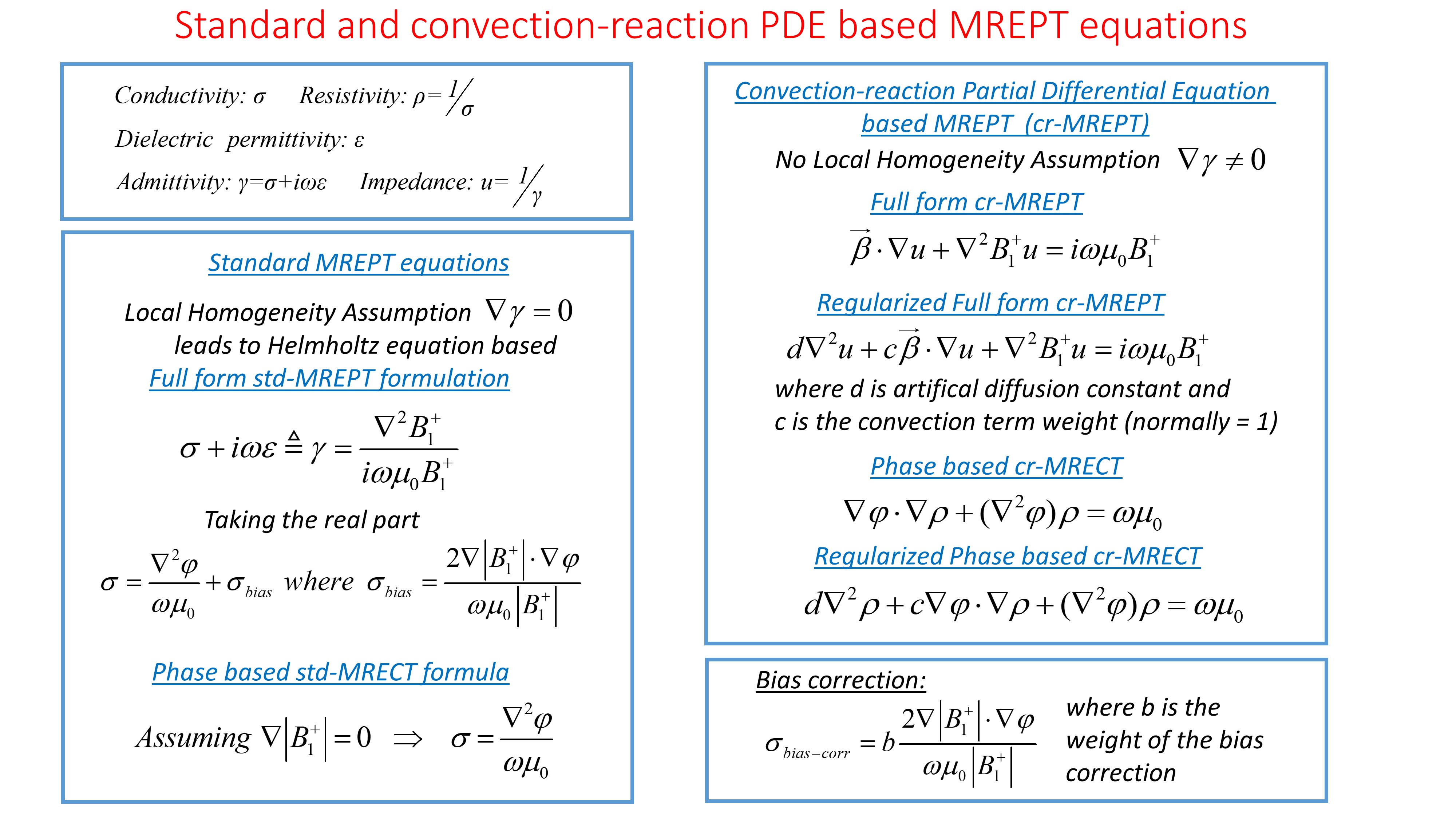
MREPT formulations are given in Figure-1. Helmholtz-equation based std-MREPT^1,2 is derived assuming homogeneous electrical properties and therefore has boundary artifacts. To circumvent this problem, cr-MREPT is developed³. In general MREPT requires the knowledge of both the magnitude and phase of $$$B_1^+$$$. Since the phase alone can be measured faster and with higher SNR, phase based versions of reconstruction, of only the conductivity however, have been developed^4,5, which also assume that $$$\triangledown\mid{B_1^+}\mid$$$ is negligible. In this work some properties and implementation issues of the Phase based cr-MRECT are studied, namely, discretization methods, ill conditioning, regularisation, bias due to the $$$\triangledown\mid{B_1^+}\mid=0$$$ assumption, and weighting of the convection term.

Methods

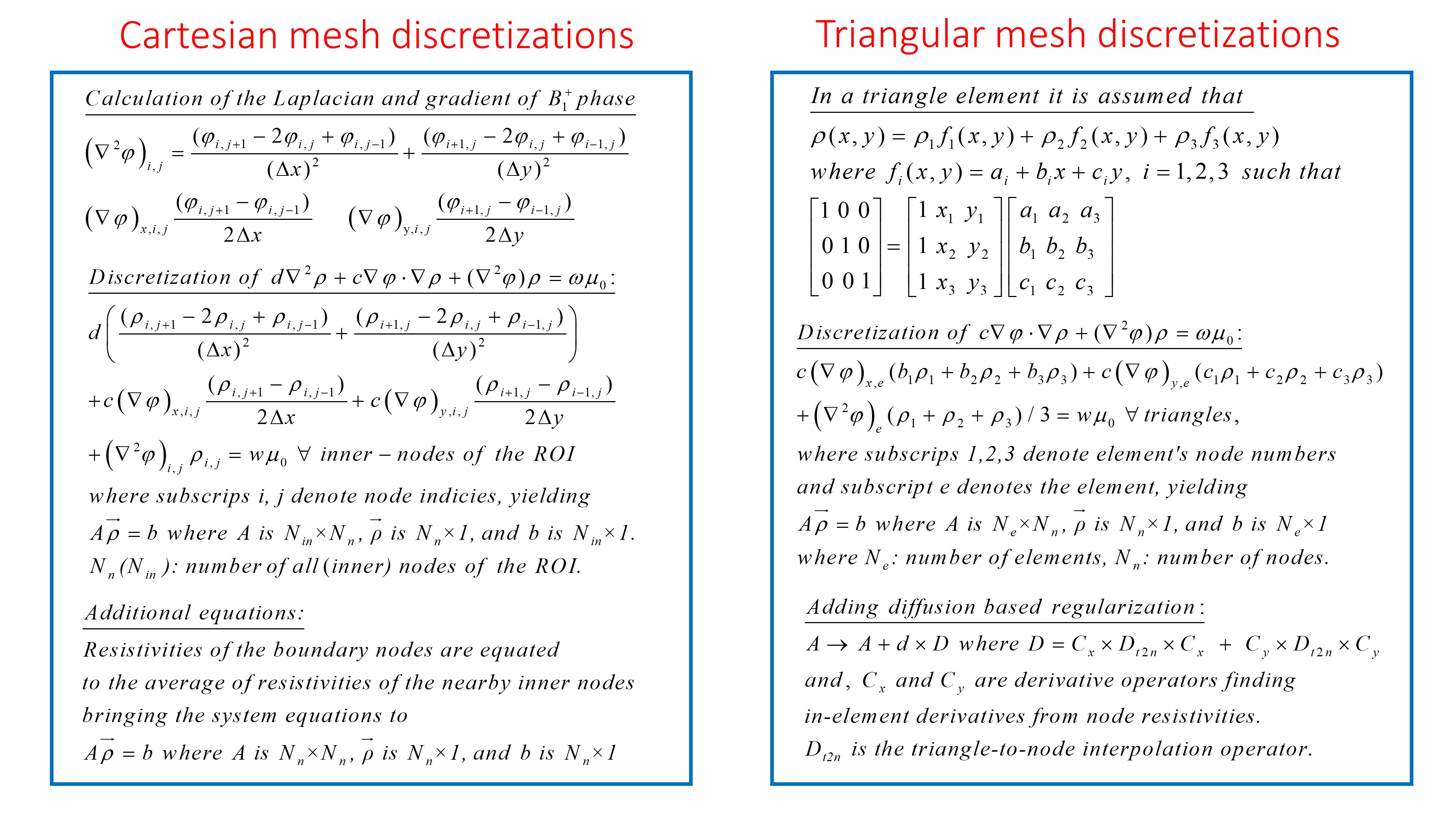
Forward problem simulations are performed using Comsol Multiphysics (COMSOL AB, Stockholm, Sweden) in a 2D setting in order not to be effected by $$$B_z$$$. A conductive phantom of 12cm diameter is placed in a square computation domain of 2m side-length, at the boundary of which the transverse magnetic field is taken to be $$$\mu_0(-iu_x-u_y)$$$, thus simulating an applied rotating magnetic field and obtaining an otherwise uniform $$$B_1^+$$$ in the place of the conductive object. Finite element method with triangular (<0.5mm) mesh is used to solve for $$$B_1^+$$$. Solution is exported to Matlab (The Mathworks, Natick, MA, USA) on a 1.5mm Cartesian grid.

Gaussian noise of $$$stdev=mean\left(\mid{B_1^+}\mid\right)/1000$$$ is added to both components of complex $$$B_1^+$$$ which is then LP filtered (3X3 Gaussian, stdev=0.5pixel). Laplacian and gradient of $$$\phi=angle(B_1^+)$$$ are calculated using the discretization formulae given in Figure-2. Region-of-Interest (ROI) is selected via mouse clicks using the “impoly” function of Matlab, such that the boundary errors due to filtering and calculation of Laplacian and gradient of $$$\phi$$$ are excluded.

Discretization of the Phase based cr-MRECT equation is implemented by (i) using the Cartesian-mesh in the ROI, and (ii) using a triangular-mesh generated in the ROI (Figure-2). The system equations are solved using the backslash operator of Matlab. No Dirichlet boundary condition is imposed.

A fourth order polynomial is fit to $$$\mid{B_1^+}\mid$$$ and then the bias correction term $$$ \sigma_{bias-corr}$$$ is calculated from the fit surface, which has the weight coefficient “b”.

Results

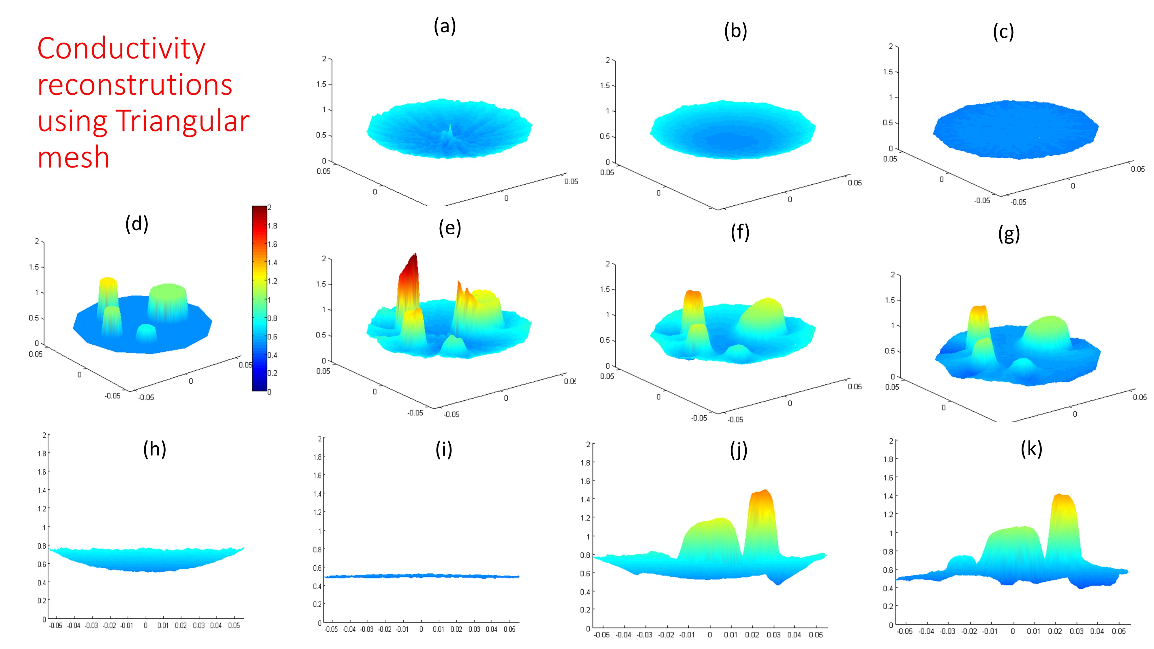
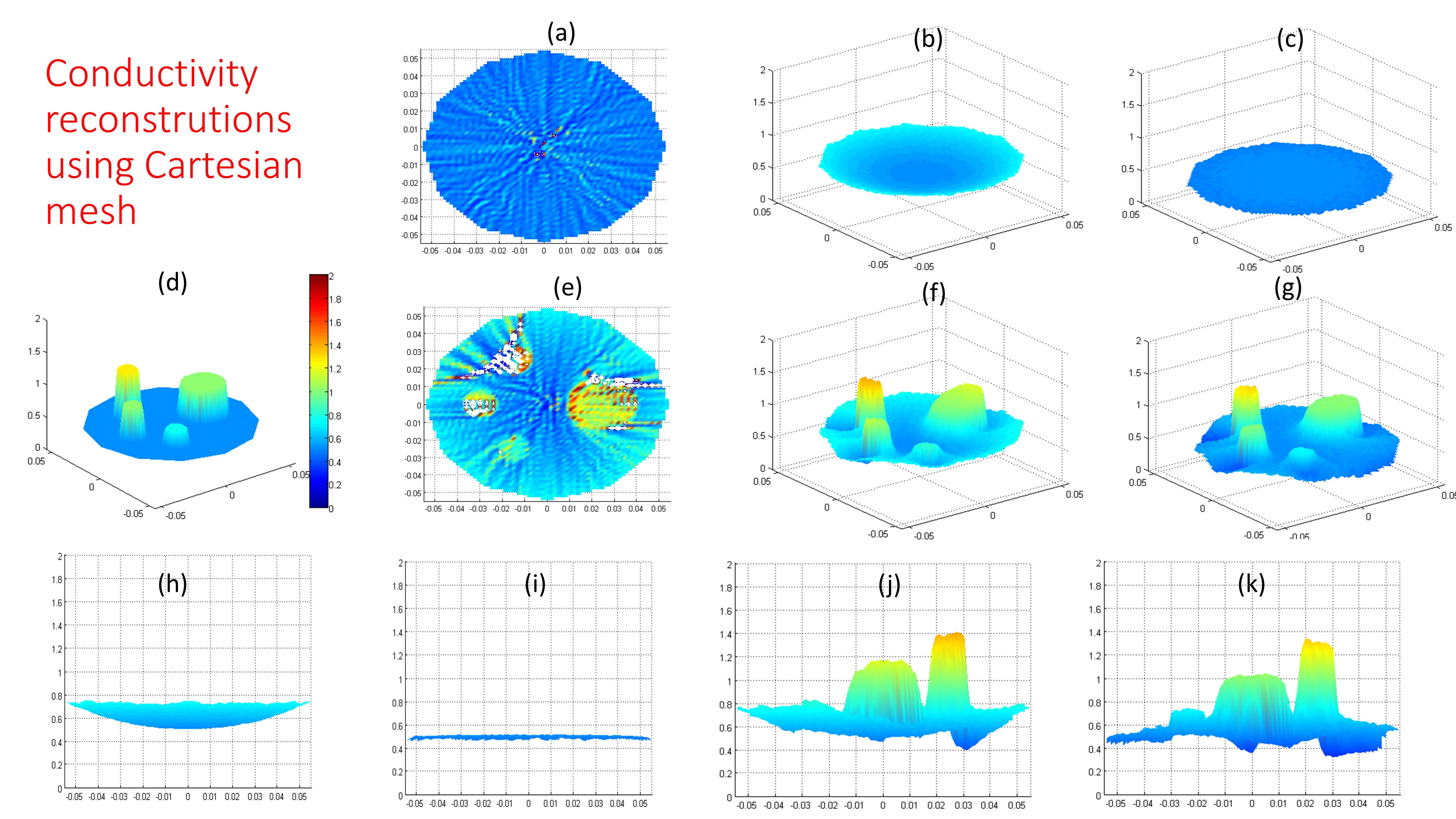
Figure-3 shows the reconstruction results using a triangular-mesh in a circular ROI of 5.5 cm radius. For a homogeneous object with sigma = 0.5 S/m, without the diffusion term (d=0), the reconstruction is noisy and more profoundly so in the Low Convective Field (LCF, $$$\triangledown\phi≈0$$$) region. With d=-0.01 however, noise and LCF artifacts disappear. Adding also the bias correction term (b=0.45), a uniform 0.5S/m image is obtained. For an object with 4 anomalies introduction of the diffusion term (d=-0.01) and adding the bias-correction term (b=0.45), clean images with no boundary artifacts are observed. Some blurring and some remains of the boundary artifacts are however observed.

Figure-4 shows the Cartesian-mesh reconstruction results for the same simulation phantoms. Most importantly, if diffusion term is not used spurious oscillations are observed around sharp edges which are however easily eliminated introducing diffusion (d=-0.01). Otherwise the results are similar to the triangular-mesh case.

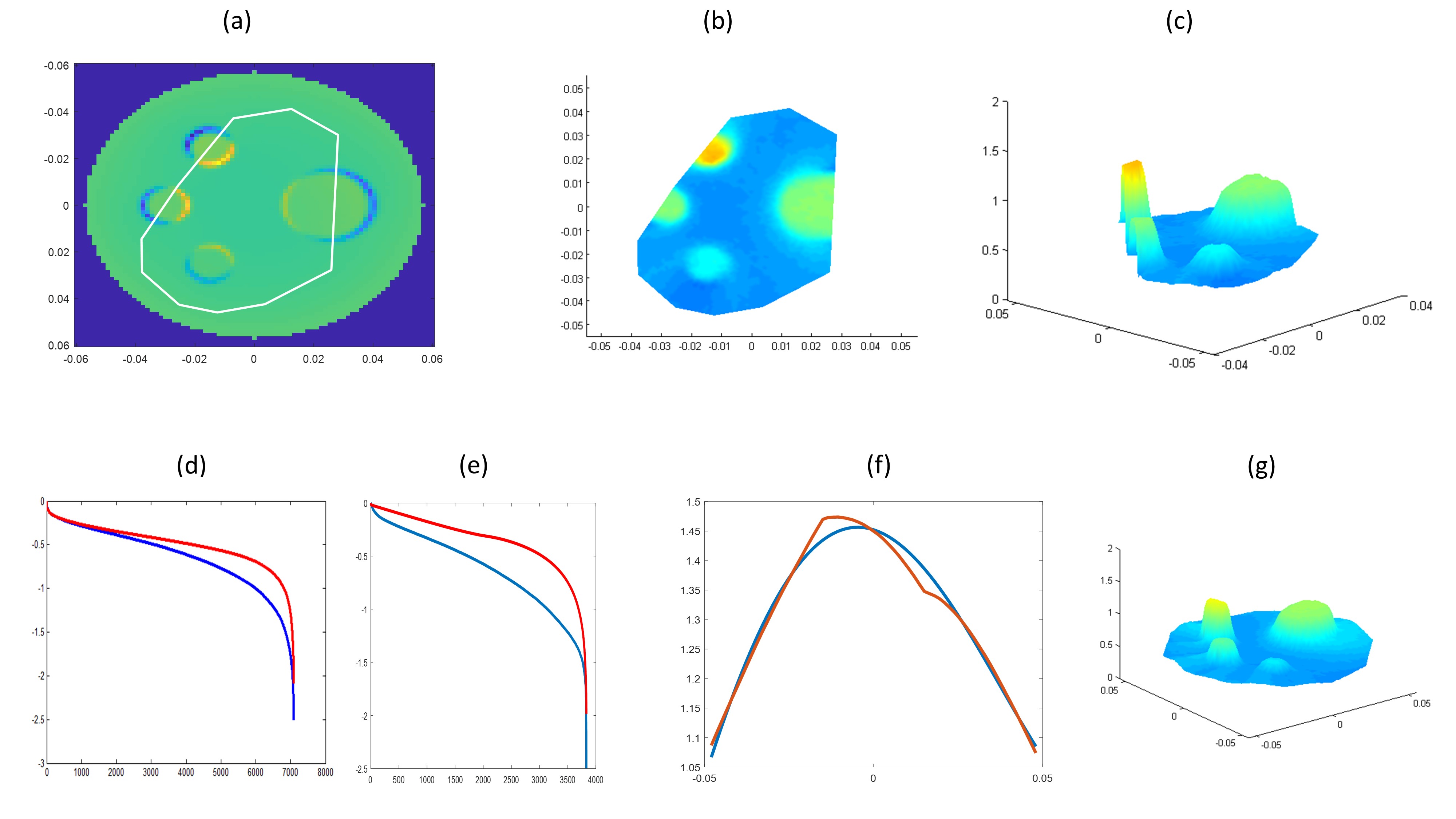
It is not necessary to impose Dirichlet boundary conditions. This is clearly evident in Figure-5, where a small ROI is selected such that the boundary of the ROI cuts several anomalies through their centers. The boundary of the ROI is accurately reconstructed.

The ill-conditioning of the system matrices are also studied as shown in Figure-5. Without diffusion, condition numbers are 325 and 313 for the Cartesian and triangular-mesh cases respectively. With diffussion these are reduced to 123 and 97 respectively.

Figure-5f shows the x=2.4mm profiles of $$$\mid{B_1^+}\mid$$$ and its polynomial fit. A 4th order polynomial fits almost perfectly to the uniform case (not shown), and for the 4-anomaly phantom, with 4th order fitting, details are omitted and the main trend is modelled.

With c=1.75 we find that the boundary correction due to the convection term is more effective as shown in Figure-5g.

Discussion and Conclusion

One important conclusion is that there is no need for specifying conductivity on the boundary of the ROI.

Since the diffusion term is in any case necessary to combat noise and LCF artifact, we therefore conclude that the Cartesian and triangular discretizations are equally applicable. More equations in the triangular case makes the solution smoother.

The fact that cr-MRECT can be applied for any ROI is important because having to apply it to the whole domain results in the handling of an unnecessarily large system matrix and also inclusion of some possibly corrupted measurements. In practice, the ROI may be selected from an image of the MR magnitude.

The bias-correction term needs to be weighted by less than 1 (b≈0.45). This is probably because while the convection term basically works for correcting the boundary artifacts, it also somewhat alters the overall bias. In practice, $$$\mid{B_1^+}\mid$$$ may be measured with a quick and low resolution method, like DREAM⁶, and the bias-correction term can be calculated by fitting a polynomial to $$$\mid{B_1^+}\mid$$$ which captures the main trend in it.

Using a somewhat higher weight for the convection term is more effective for combatting the boundary artifacts. However the bias is also effected and the bias-correction weight must also be adjusted (as future work).

Acknowledgements

No acknowledgement found.