3187
Experimental Validation of Conductivity Tensor Imaging using Giant Vesicle Suspension
In Ok Ko1, Bup Kyung Choi2, Nitish Katoch2, Ji Ae Park1, Yong Soo Cho3, Jin Woong Kim3, Hyung Joong Kim2, and Eung Je Woo2
1Korea Institute of Radiological and Medical Sciences, Seoul, Korea, Republic of, 2Kyung Hee University, Seoul, Korea, Republic of, 3Chosun University Hospital and Chosun University College of Medicine, Gwangju, Korea, Republic of
1Korea Institute of Radiological and Medical Sciences, Seoul, Korea, Republic of, 2Kyung Hee University, Seoul, Korea, Republic of, 3Chosun University Hospital and Chosun University College of Medicine, Gwangju, Korea, Republic of
Synopsis
Conductivity tensor can realize volume conductor model of brain for neuroimaging and electrical stimulation. We report validation of electrodeless conductivity tensor imaging (CTI) method [1]. From CTI imaging using giant vesicle suspension at 9.4T MRI, relative error in conductivity tensor image was found to be less than 1.7% compared with the measured values using an impedance analyzer. High- and low-frequency conductivity can quantify total and extracellular water contents, respectively, at every pixel. Their difference can quantify intracellular water content at every pixel. Current CTI method can separately quantify the contributions of ion concentrations and mobility to the conductivity tensor.
Purpose
The purpose of this study is to validate the performance of the CTI method to produce low-frequency conductivity tensor images using a conductivity phantom including a giant vesicle suspension.Methods
Giant vesicles dispersed in aqueous solution were prepared as described by Moscho et al. [2]. 2 ml of phospholipids dissolved in chloroform with a concentration of 30 mg/ml was added to a 1 liter round-bottom flask containing 3 ml of chloroform and 400 μm of methanol. The handling of phospholipids was proceeded only under argon atmosphere. Distilled water or 0.75 % NaCl solution in a volume of 20 ml was carefully added not to disturb the interface between the aqueous phase and organic solution phase. The round-bottom flask was installed to a rotary evaporator to remove organic solvent at 47 °C under vacuum with nitrogen trap for 20 min at 10 rpm and then followed by another 20 min at 60 rpm. During evaporation of organic solvents, phospholipids in organic solution trapped in the saline phase and assembled to form giant vesicles. The resultant aqueous solution containing giant vesicles was subjected to centrifugation at 1,500 rpm for 10 min. The volume fraction of the giant vesicles after the centrifugation was about 80 to 90 % by visual observations. The mean and standard deviation (SD) of the diameters of the giant vesicles were 13 ± 4.7 μm. A 9.4T MRI scanner was used for imaging experiments. The high-frequency conductivity images were acquired using the multi-echo spin-echo sequence with an isotropic voxel resolution of 0.5 mm. The imaging parameters were as follows: TR/TE = 2200/22 ms, number of signal acquisitions = 5, field-of-view (FOV) = 65 × 65 mm2, slice thickness = 0.5 mm, flip angle = 90, and image matrix size = 128 × 128. Six echoes were acquired with the total scan time of 23 min. Diffusion weighted MR imaging was separately performed using the single-shot spin-echo echo-planar-imaging sequence. The imaging parameters were as follows: TR/TE = 2000/70 ms, number of signal acquisitions = 2, FOV = 65 × 65 mm2, slice thickness = 0.5 mm, flip angle = 90, and image matrix size = 128 × 128. The number of directions of the diffusion-weighting gradients was 30 with 15 b-values.Results and Discussion
Fig. 1(b) shows the intermediate variables including the high-frequency conductivity σH, extracellular volume fraction χ, extracellular water diffusion coefficient dew, intracellular water diffusion coefficient diw, and scale factor η where the relation between the conductivity tensor C and the extracellular water diffusion tensor Dew is given by C = ηDew [1]. Fig. 1(c) is the image of Dew estimated by the CTI method [1] and (d) shows the reconstructed CTI image. Table 1 shows the mean and standard deviation of the intermediate variables and the diagonal components Cxx, Cyy, and Czz. These values were computed from all pixels within each region. The value of σH measured in the CTI framework at 400 MHz (Larmor frequency at 9.4 T) were 1.86 ± 0.04 and 1.11 ± 0.04 S/m in the electrolytes #1 and #2, respectively. In the giant vesicle suspension, σH was 1.89 ± 0.02 S/m. The value of χ in both electrolyte regions was 1.00 ± 0.02 as expected. The value of χ in the giant vesicle suspension was 0.13 ± 0.04, which was in good agreement with the visually observed value after the giant vesicles were concentrated by centrifugation. The value of dew in the electrolytes #1 and #2 were 2.90 ± 0.01 and 2.85 ± 0.02 μm2/ms, respectively, which are close to the free water diffusion coefficient. The value of diw in the electrolytes #1 and #2 were meaningless since they contained no cells. In the giant vesicle suspension, dew was 1.93 ± 0.12 μm2/ms indicating that water diffusion in the extracellular space of the giant vesicle suspension was hindered by the closely packed giant vesicles. The value of diw in the giant vesicle suspension was 0.98 ± 0.10 μm2/ms. Considering that the average diameter of the giant vesicles was 13 μm, the small value of diw should have stemmed from the restricted water diffusion [3] inside the giant vesicles. Multiplying η to the diffusion tensor Dew at each pixel, the image of the conductivity tensor C in Fig. 1 was reconstructed. Cxx, Cyy, and Czz in the giant vesicle suspension region were 0.29 ± 0.05, 0.30 ± 0.07, and 0.29 ± 0.05 S/m, respectively. The reconstructed high- and low-frequency conductivity values from the CTI were marked Fig. 2 for comparisons by using the impedance analyzer.Conclusion
The performance of the CTI method to produce low-frequency conductivity tensor images is validated using a conductivity phantom including a giant vesicle suspension. Note that the high-frequency and low-frequency conductivity values are correlated with the total and extracellular water contents, respectively, at every pixel. The difference between them is correlated with the intracellular water content at every pixel. In addition, the CTI method can quantitatively separate the contributions of ion concentrations and mobility to the conductivity tensor at every pixel .Acknowledgements
This work was supported by the National Research Foundation of Korea (NRF), the Ministry of Health and Welfare of Korea, and Korea Institute of Radiological and Medical Sciences (KIRAMS) grants funded by the Korea Government (2018R1D1A1B07046619, 2019R1A2C2088573, HI18C2435, and 50461-2019).References
- S. Z. K. Sajib et al. Electrodeless conductivity tensor imaging (CTI) using MRI: Basic theory and animal experiments. Biomed. Eng. Lett. 2018;8:273–282.
- A. Moscho et al. Rapid preparation of giant unilamellar vesicles. Proc. Nat. Acad. Sci. 1996; 93:11443–11447.
- P. N. Sen et al. Time-dependent diffusion coefficient as a probe of geometry. Concepts Magn. Reson. 2004;23A:1–21.
Figures
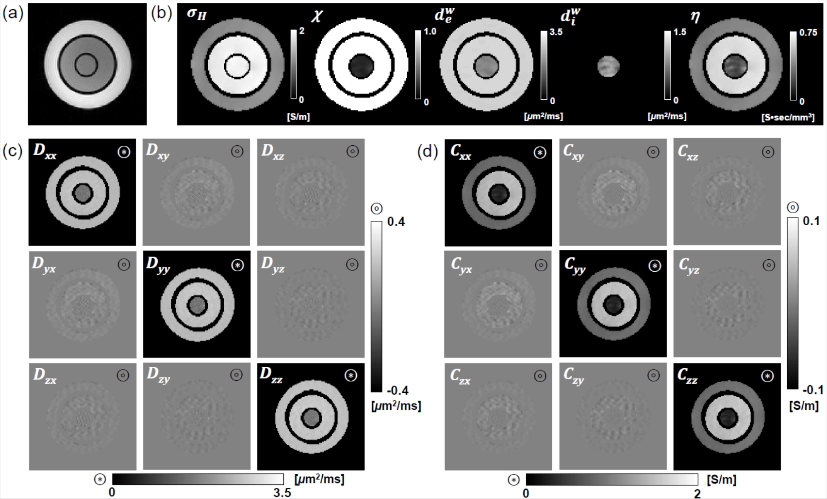
Fig. 1. Reconstructed CTI images of the conductivity phantom.
(a) T2 weighted image. (b) Images of the high-frequency conductivity σH, extracellular volume
fraction χ, extracellular water
diffusion coefficient dew, intracellular water
diffusion coefficient diw and scale factor η between the conductivity tensor
and the water diffusion tensor. (c) Water diffusion tensor image. (d)
Conductivity tensor image.
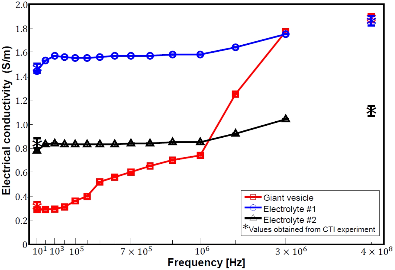
Fig. 2. Conductivity spectra of two electrolytes and the giant
vesicle suspension from 10 Hz to 3 MHz. The values recovered from the CTI
experiments were plotted as asterisks at 10 Hz and 400 MHz.
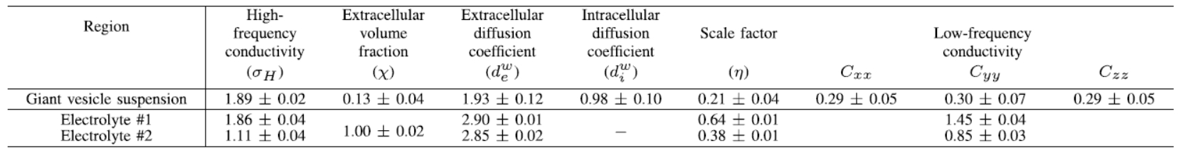
Table.
1. Mean and standard deviation values of the diagonal components of the conductivity
tensor C and the intermediate variables including the high-frequency
conductivity σH, extracellular volume fraction χ, extracellular
water diffusion coefficient dew, intracellular water diffusion coefficient diw, and scale factor η. The mean ± SD values were
computed from all pixels within each region.