Introduction

In magnetic resonance electrical properties tomography (MREPT), the EPs are reconstructed via measuring the positive circularly polarized component, $$$H^+=(H_x+iH_y)/2$$$, corresponding to the radio-frequency (RF) excitation, while the negative circularly polarized component, $$$H^-=(H_x-iH_y)/2$$$, is usually ignored in reconstruction. However, depending on EP distribution, it is pointed out¹ that the reconstruction error, when neglecting $$$H^-$$$, increases roughly to 3-4% in simulations and 10% in phantom experiments. In this study, we derive a simple formula to compute $$$H^-$$$ from the measured $$$H^+$$$. As a result, we can separately determine $$$H_x$$$ and $$$H_y$$$ from the measured $$$H^+$$$ and computed $$$H^-$$$. We show that the obtained $$$H_x$$$ and $$$H_y$$$ can be used in a regularization term for EP reconstruction, which can suppress the instability of reconstruction at the low convection field (LCF) region where the $$$z$$$-component of the electric field is close to zero.

Theory

Assuming that $$$H_z = 0$$$, Faraday’s law can be represented as
$$\bar{\partial}E_z-\partial_zE^+=\omega\mu_0H^+,\cdots\hbox{(1)}\qquad\partial E_z-\partial_z E^-=- \omega\mu_0 H^-,\cdots\hbox{(2)},\qquad\partial E^+-\bar{\partial}E^-=0,\cdots\hbox{(3)}$$
where $$$\partial=(\partial_x-i\partial_y)/2, \bar{\partial}=(\partial_x+i\partial_y)/2, E^+=(E_x+i E_y)/2,\, \hbox{and}\,E^-=(E_x-iE_y)/2$$$. Note that Equations (1) and (2) are obtained from ($$$x$$$-component) $$$\pm\,i$$$ ($$$y$$$-component) of Faraday’s law. Assume further that $$$|\partial_zE^+| \ll |\bar{\partial}E_z|, \quad |\partial_zE^-| \ll |\partial E_z|$$$, which holds when the $$$z$$$-derivative of the EPs is sufficiently smaller than the $$$x$$$- and $$$y$$$-derivatives, then, Equations (1) and (2) turn into
$$\bar{\partial}E_z=\omega\mu_0H^+,\cdots\hbox{(4)},\qquad\partial E_z=-\omega\mu_0 H^-.\cdots\hbox{(5)} $$.
Equation (4) is the so-called Dbar equation and can be solved using the generalized Cauchy formula as² $$E_{z}(w)=-\frac{1}{2\pi i}\int_{\partial\Omega}\frac{4\,\lambda\,\partial H^+(\zeta)}{\zeta-w}d\zeta-\frac{\omega\mu_0}{\pi}\int\int_\Omega\frac{H^+(\zeta)}{\zeta-w}d\xi d\eta,\cdots\hbox{(6)}$$
where $$$\lambda=1/\gamma$$$ with $$$\gamma=\sigma+i\omega\epsilon$$$, $$$\sigma$$$ and $$$\epsilon$$$ are the electrical conductivity and permittivity, respectively, $$$\zeta=\xi +i\eta$$$, and $$$\Omega$$$ is a region of interest (ROI). Thus, substituting Equation (6) into (5) leads to our main result of this study:
$$H^-(w)=\frac{1}{\omega\mu_0}\left(\frac{1}{2\pi}\int_\Gamma\frac{4\lambda\partial H^+(\zeta)}{(\zeta-w)^2}d\zeta+\frac{1}{\pi}\int\int_\Omega\frac{\omega\mu_0 H^+(\zeta)}{(\zeta-w)^2}d\xi d\eta\right).\cdots\hbox{(7)}$$
Equation (7) tells us how to compute $$$H^-$$$ from the measured $$$H^+$$$ in the ROI and the boundary value of $$$\lambda$$$. From $$$H^-$$$ and $$$H^+$$$, $$$H_x$$$ and $$$H_y$$$ are separately obtained.

Let us now consider Ampere’s law represented as
$$i\lambda\partial_z H^+=E^+\cdots\hbox{(8)},\quad-i\lambda\partial_zH^-=E^-\cdots\hbox{(9)},\quad-4i\lambda\partial H^+=E_z.\cdots\hbox{(10)}.$$ In our previous paper², we used Equations (6) and (10) to determine $$$\lambda$$$. Note that Equations (3), (8) and (9) have not been used so far for MREPT. Substituting Equations (8) and (9) into (3), noting that div $$$\bf{H}$$$ = 0, we have
$$\partial_zH_x\partial_x\lambda+\partial_zH_y\partial_y\lambda=0\cdots\hbox{(11)}$$
stating that the gradient of $$$\lambda$$$ should be always orthogonal to the $$$z$$$-derivatives of $$$H_x$$$ and $$$H_y$$$. This physical constraint can be used for the regularization in the reconstruction of EPs. We minimize the cost function$$||Ax-b||^2+\alpha^2||(FD_x+GD_y)x||^2,\cdots\hbox{(12)}$$
where $$$x$$$, $$$A$$$, $$$b$$$, $$$F$$$ and $$$G$$$ are composed of appropriately aligned $$$\lambda$$$, $$$-4i\partial H^+$$$, $$$E_z$$$ (with some constants), $$$\partial_z H_x$$$ and $$$\partial_z H_y$$$ at each point of the ROI, and $$$D_x$$$ and $$$D_y$$$ represents the $$$x$$$- and $$$y$$$-derivatives.

The proposed method was verified numerically. A numerical model of a 16-leg, high-pass shielded birdcage coil with a diameter of 240 mm and height of 270 mm was formulated. The magnetic field at 123.2MHz was generated in a quadrature excitation model. The ROI was a 90mm by 90mm square region centered at the origin in the $$$xy$$$-plane. The sample points were taken at 64 by 64 points. As a numerical phantom, a cylinder with a diameter of 144mm, height of 270mm, electrical conductivity of 0.5S/m, and relative permittivity of 50 was assumed. Inside it, three cylinders mimicking malignant tissues were inserted whose radii were 15mm, 10mm, and 5mm. All of these cylinders were 15 mm in height and they were located at -12.5mm $$$<z<$$$ 2.5mm. Note that the EP discontinuously changed at $$$z=0$$$. $$$H^+$$$ was computed using the FEM software, COMSOL Multiphysics 5.2a (COMSOL Inc.). Gaussian noise were added to the magnitude and phase of $$$H^+$$$ where their standard deviations were 0.1% of those of the theoretical data. The first order spatial derivative of $$$H^+$$$ was computed using the Savitzky-Golay filter. Although the area integral in Equation (7) seems singular, it can be shown that the integral over a circle centered at $$$w$$$ with a radius $$$\epsilon$$$ is proportional to $$$\epsilon^2$$$. From this, we simply removed the integrand value at the pixel including $$$w$$$. The regularization parameter $$$\alpha$$$ is given by the ratio of the largest singular value of $$$A$$$ to that of $$$FD_x+GD_y$$$.

Results and Discussion

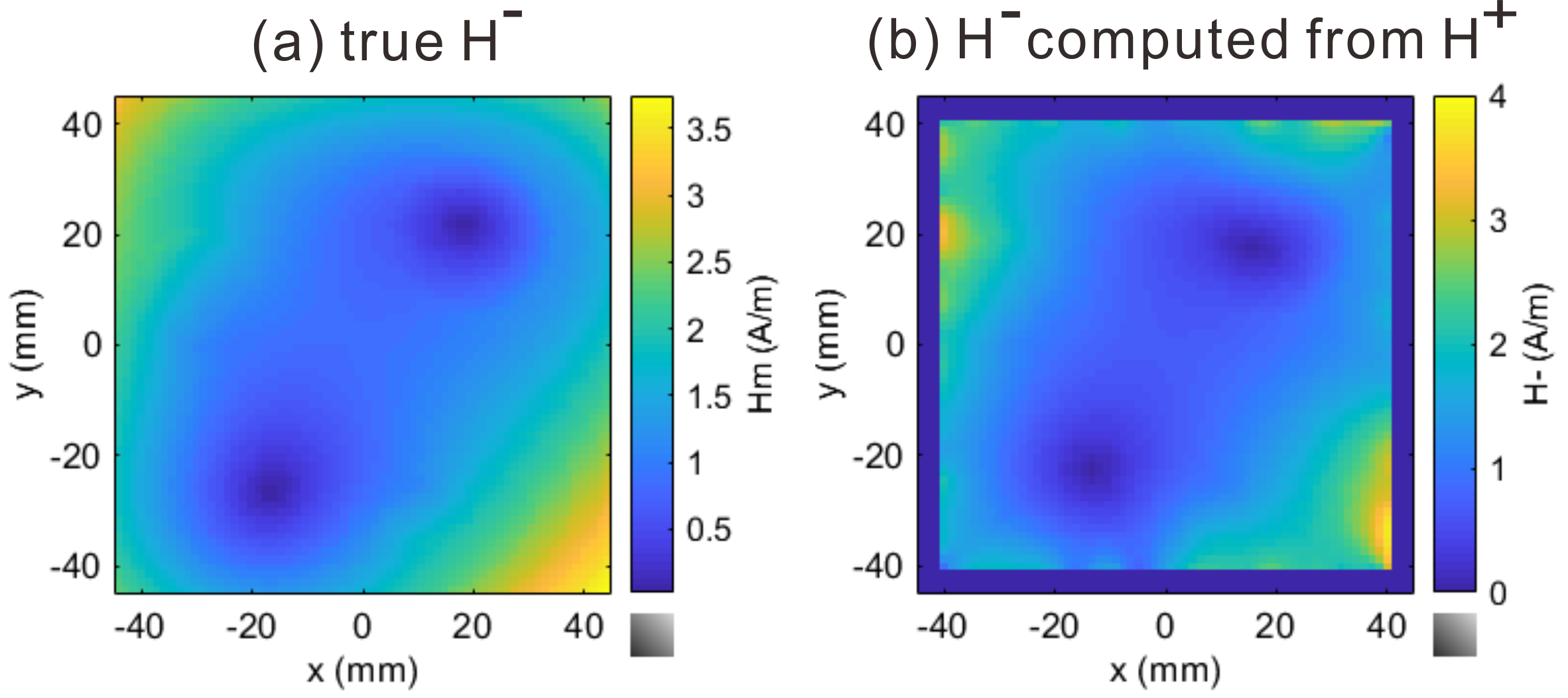
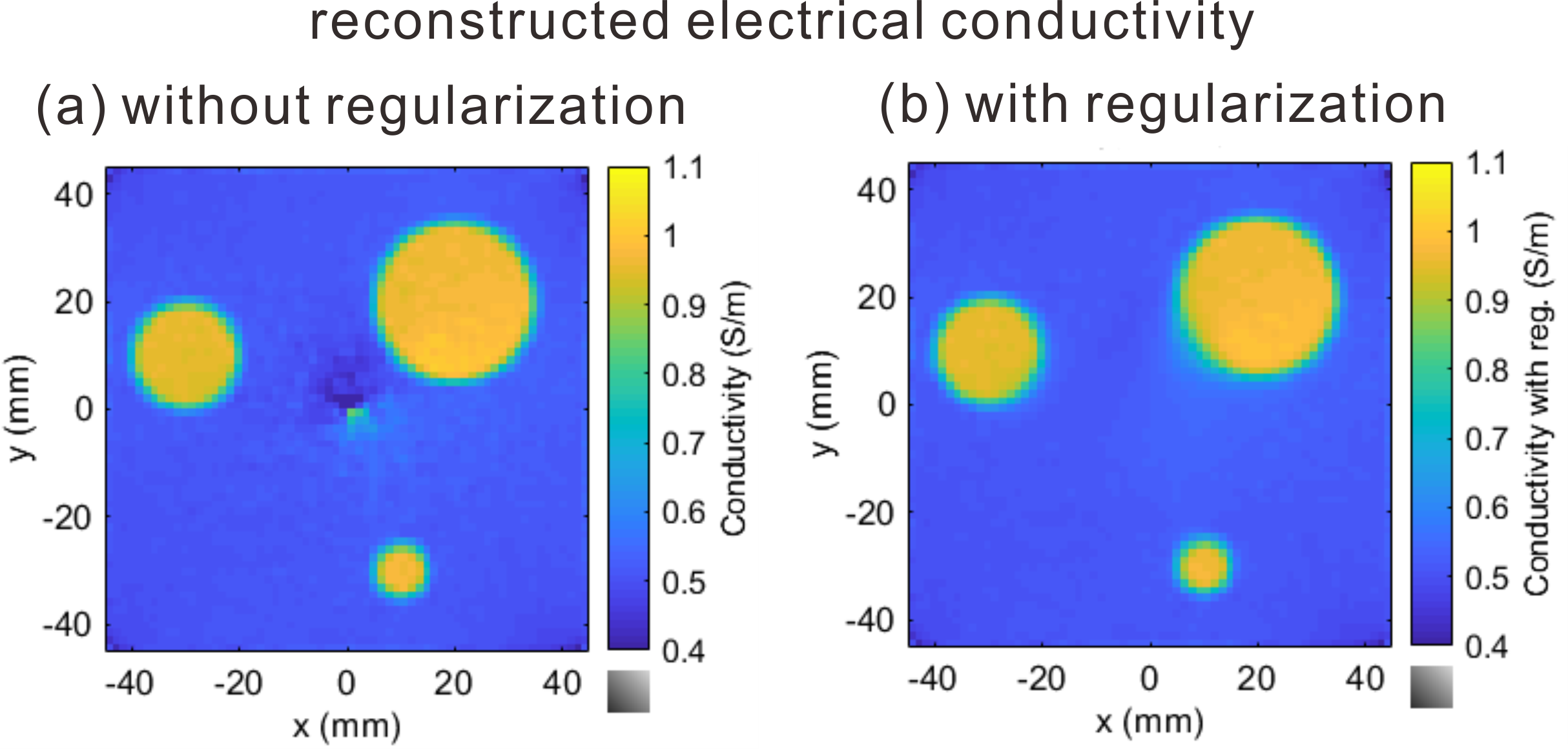
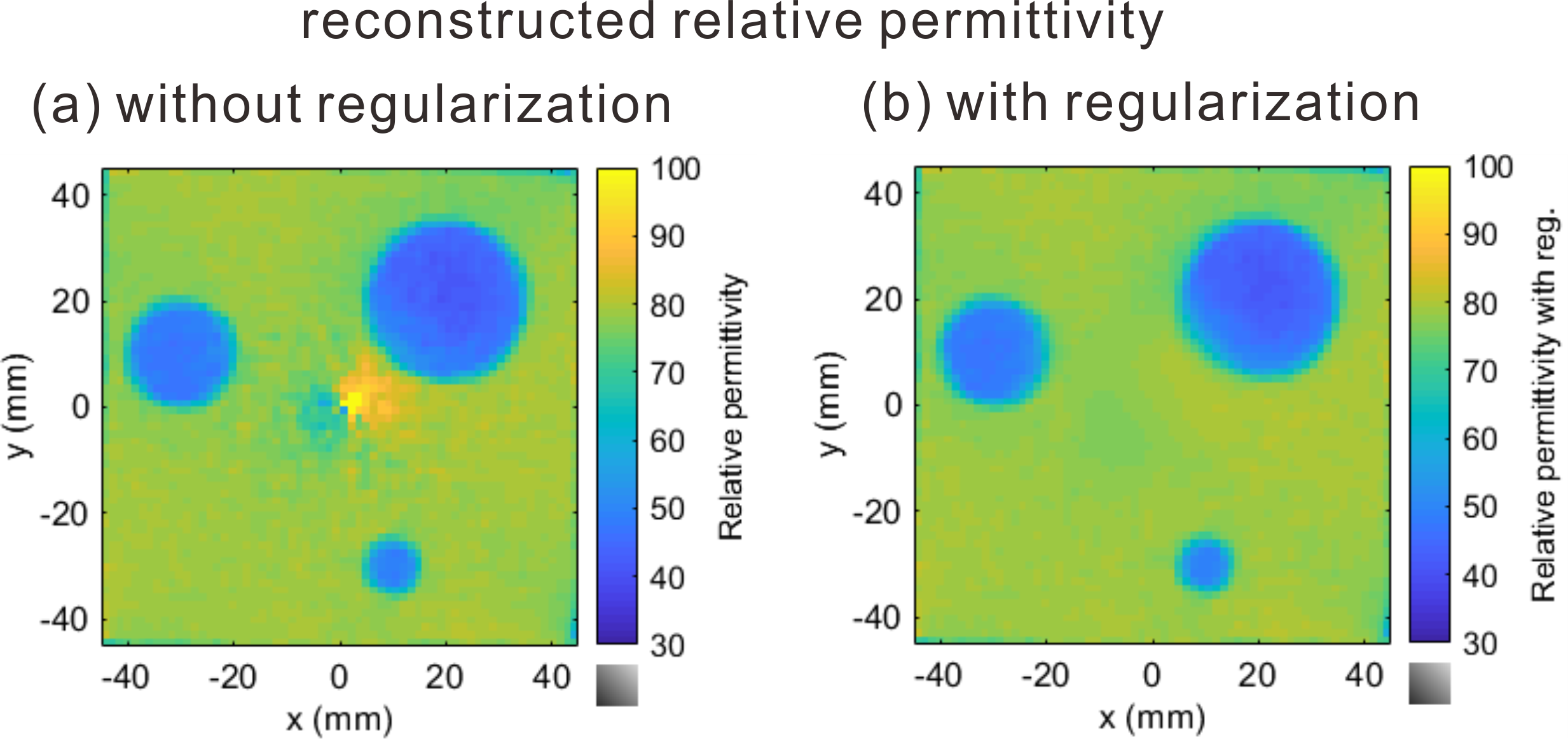
The left and right panels of Figure 1 show the true and computed values of $$$H^-$$$. We observe that $$$H^-$$$ can be well computed using Equation (7) except near the boundary of the ROI. Two lines adjacent to the boundary are not shown in order to compare the true and estimated values around the origin. The inaccuracy near the boundary is due to the kernel $$$1/\zeta^2$$$, which has a large amplitude there. The left and right panels of Figure 2 show the reconstructed conductivity without and with regularization. Figure 3 illustrates the result of the relative permittivity. We observe that the regularization term with nonzero $$$\alpha$$$ suppresses the artifact due to LCF.

Conclusion

We derived an explicit formula to compute $$$H^-$$$ from the measured $$$H^+$$$ with the boundary values of EPs when the amplitudes of the $$$z$$$-derivatives of the electric field are much smaller than the $$$x$$$- and $$$y$$$-derivatives. From the obtained $$$H^-$$$, a new regularization term was proposed which suppresses the artifact generated at the LCF region.

Acknowledgements

This research was partly supported by JPSP KAKENHI Grant Number 19H04438 and Canon Medical Systems Corporation.