3184
Conductivity Tensor Imaging (CTI): a novel contrast mechanism based on ionic conductivity for characterization of brain tumors1Department of Biomedical Engineering, Kyung Hee University, Seoul, Republic of Korea, 2Physiology, University of Liverpool, Liverpool, United Kingdom, 3School of Engineering, Macquarie University, Sydney, Australia
Synopsis
Unlike the previously reported method of diffusion tensor magnetic resonance electrical impedance tomography (DT-MREIT), conductivity tensor imaging (CTI) does not require external electrodes for current injection. The low frequency conductivity (σL) value can be estimated from the high frequency conductivity (σH) measured using B1 map. The σL is influenced by cell size and density, which makes it an effective technique to characterize the cellular changes in brain tumors. Rat brain tumors were studied using 9.4 T MRI scanner using CTI protocol. Changes in ionic concentration cellular states depending on tumor growth were reflected in both high and low-frequency CTI images.
Purpose
The purpose of this study was to test the efficacy of CTI in the characterization of an intracranial model of rat gliomas at ultra-high magnetic fields of 9.4T with a spatial resolution of 300x300x300 µm3.Methods
Conductivity Tensor Imaging (CTI) has recently been proposed as a novel method to image anisotropic conductivity of brain tissues at low frequencies1,2. Unlike the previous method of diffusion tensor magnetic resonance electrical impedance tomography (DT-MREIT), it does not require external electric current to probe body for conductivity measurement1-3. To explore the potential of CTI for low-frequency conductivity mapping, orthotopic glioblastomas models were studied. The tumors were induced by transcranial injection of F98 cells in the right cortex. Six F344 female (100-120 g) rats were injected with 50,000 F98 cells suspended in 5 µL PBS solution. The image of the conductivity tensor was reconstructed using CTI formula1,2. $$C=D_e^w(χσ_H)/(χd_e^w+(1-χ)d_i^wβ)=ηD_e^w$$ where, $$$σ_H$$$ is the high-frequency conductivity at the Larmor frequency, χ is the extracellular volume fraction, β is the ion concentration ratio of intracellular and extracellular spaces, $$$d_e^w$$$ and $$$d_i^w$$$ are the extracellular and intracellular water diffusion coefficients, η is position dependent scale factor and $$$D_e^w$$$ is the extracellular water diffusion tensor. Longitudinal MRI, including DTI and MREPT was performed on 8th, 11th and 14th day after tumor cell implantations. The multi-echo spin-echo pulse sequence with multiple refocusing pulses was adopted to obtain the B1 phase map for reconstruction of high-frequency conductivity ($$$σ_H$$$). The imaging parameters were as follows: TR/TE = 4341/8 ms, number of echoes = 10, NEX = 2, slice thickness = 300 µm, number of slices = 38, matrix size = 128×64, and FOV = 40×20 mm2. Multi-b value diffusion weighted imaging data sets were obtained using the single-shot spin-echo echo-planar-imaging pulse sequence to calculate, χ, $$$d_e^w$$$, $$$d_i^w$$$ and $$$D_e^w$$$. The number of directions of the diffusion-weighting gradients was 20 with b-values of 50, 150, 300, 500, 700, 1000, 1400, 1800, 2200, 2600 and 3000 s/mm2, TR/TE = 2500/23 ms, slice thickness = 0.3 mm, flip angle = 90°, number of excitations = 5, number of slices = 38 and acquisition matrix = 128×64. An additional conventional T2 weighted scan of 5 minutes was also acquired for anatomical reference. The parameter β was set to the value of 0.41 as suggested in1. The $$$σ_H$$$ and $$$σ_L$$$ images were co-registered with T2-weighted images and mean values were extracted by drawing ROI over the tumor region, pointed by arrows and marked by red colored boundaries in T2 images of figure 1.Results
Figure 1 shows the T2-weighted images, high frequency ($$$σ_H$$$) conductivity, and low frequency ($$$σ_L$$$) conductivity images from top to bottom row, respectively. The images cover the tumor from a representative rat showing the variation of $$$σ_H$$$ and $$$σ_L$$$ from left to right columns for 8th, 11th and 14th day after tumor cell implantations. The low-frequency conductivity images shown in figure 1 are isotropic, represented as $$$σ_L=(Cxx+Cyy+Czz)/3$$$, where $$$Cxx$$$, $$$Cyy$$$ and $$$Czz$$$ are the diagonal component of conductivity tensor. The mean and standard deviations of σH and σL in tumor regions were compared across these days in table 1. The $$$σ_L$$$ values are lower than $$$σ_H$$$ values as was reported in earlier study4. Both of $$$σ_H$$$ and $$$σ_L$$$ values from the tumour increased over time. The conductivity was higher in the ventricles and the tumor compared to the contralateral healthy brain (Table 1). The low frequency conductivity measurements were compared to the high frequency values in the same volumes-of-interest longitudinally 8, 11, and 14 days (Table 1). There was significant increase (p<0.05) in conductivity values of the tumor compared to the normal brain, reflecting changes in tumor ionic concentration, which is also reported in Na-MRI of brain tumors indicating an imbalance in the Na+/K+ pumps.Discussions
High frequency conductivity using B1 maps produces absolute conductivity distribution combining the intra and extracellular information in microscopic voxel. However, the low frequency conductivity depends upon ion concentration and mobility of charge carriers in the extracellular space only. The visualization of low frequency conductivity added the information of cell size, density, and swelling. Note that the bright contrast in edematous area is probably due to higher fluid content. The values of conductivity are almost similar in edema for low and high frequency due to the absence of tumor cells. The lower contrast and values of conductivity in σL at central part of tumor can be attributed to the increase in tumor cell density which appears in high frequency conductivity as it provides contrast information from both intra as extracellular spaces. The distinct contrast information of high and low frequency conductivity can be helpful in better characterization of tumor as well as the treatment monitoring.Conclusion
Unlike other imaging modalities CTI can provide conductivity weighted images without any additional hardware requirement. The intermediate variables of CTI such as extracellular volume fraction (χ) and intra-extra diffusion coefficients ($$$d_e^w$$$,$$$d_i^w$$$) provide the information of mobility and diffusivity which can be helpful for assessing the tumour microenvironment.Acknowledgements
References
[1] Sajib SZK “Electrodeless conductivity tensor imaging (CTI) using MRI: basic theory and animal experiments”. BELs s13534 (2018).
[2] Katoch N. “Conductivity tensor imaging of in-vivo human brain and experimental validation using giant vesicle suspension”. IEEE TMI 38, 1569-1577 (2019).
[3] Chauhan M. “Low-Frequency Conductivity Tensor Imaging of the Human Head In Vivo Usin g DT-MREIT: First Studys.” IEEE TMI 37, 966-976 (2018).
Figures
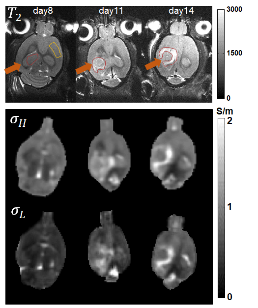
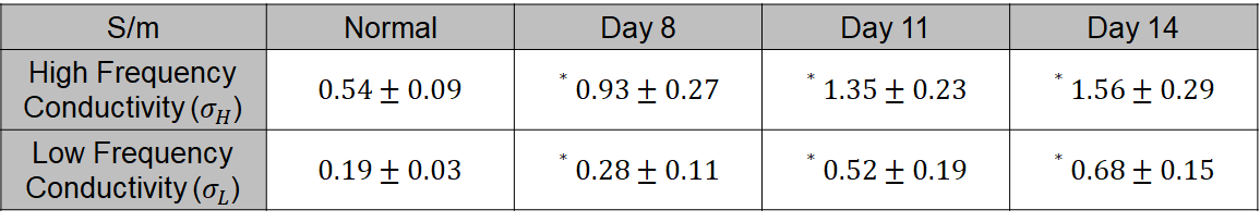
Table 1. Conductivity values obtained from CTI at high frequency ($$$σ_H$$$) and low frequency ($$$σ_L$$$) measured on 8, 11 and 14 days after tumor implantation. The * mark indicates that the values were significantly different than the normal values (p < 0.05).