3181
Machine learning methods applied to MR-based Electrical Properties Tomography to improve noise robustness and boundary accuracy.1Department of Medical Engineering, Chiba University, Chiba, Japan, 2Department of Surgery, National University of Singapore, Singapore, Singapore, 3Engineering Product Development, Singapore University of Technology and Design, Singapore, Singapore, 4Department of Radiotherapy, University Medical Center Utrecht, Utrecht, Netherlands, 5Computational Imaging Group for MR diagnostic & therapy, University Medical Center Utrecht, Utrecht, Netherlands, 6Center for Frontier Medical Engineering, Chiba University, Chiba, Japan
Synopsis
MREPT is a technique used to non-invasively estimate the electrical properties (EPs) of tissues based on Maxwell equations from MRI measurements. However, most reconstruction techniques are susceptible to noise and have severe boundary artifacts. In this work, we designed problem-oriented machine learning methods to improve the MREPT reconstructions. Through numerical experiments with 2-D cylindrical phantoms and comparison with cr-EPT, we demonstrate the feasibility of ML approaches to provide more noise robust EPT reconstructions with lower boundary artifacts.
Introduction
Magnetic resonance electrical properties tomography (MREPT) relies on Maxwell’s equations to reconstruct the electrical properties (EPs) non-invasively. To reconstruct EPs, spatial derivatives of measured B1 field (RF field) need to be computed [1]. However, derivative calculations lead to boundary errors and noise amplification [1-4]. Machine learning (ML) ability to produce application specific noise cancelling effects with high accuracy [5-6] can be helpful in MREPT reconstruction. Recently, it was shown that ML-based MREPT reconstructions are feasible [7]. In this work, we propose to address MREPT reconstruction limitations, i.e. noise amplification and boundary errors [8], with problem-oriented ML techniques.Methods
To train the neural networks (NNs), a 214 samples dataset was used. This dataset consisted of 81 solid, 169 two-layered and 64 three-layered cylindrical phantoms of different radius (Fig. 1 A). A birdcage coil working at 128 MHz was used to illuminate the phantoms using FEM-based software Comsol Multiphysics® (Fig. 1 B). Different values of EPs in the range of the human body [9] were selected (Fig. 1 C). Five B1+-maps from the center of the coil were extracted and used as inputs. To increase the number of samples, each sample was cropped into 4 equally spaced squares. The NNs trained on 70% of samples, while 30% were used for validation of the trained parameters for 500 epochs. All ML models include a convolutional noise layer to add noise (standard deviation = 0.2) during training to provide noise robustness. The NN with the highest accuracy in validation was then employed for testing. For testing, we used 5 samples that were excluded from the training/validation datasets. To test noise-robustness, the test samples were corrupted with Gaussian noise leading to SNR = 100, 50, and 25. Two ML networks were investigated to address the MREPT limitations: 1) Fully connected (FC) method [10], where we utilize a pure neural network. 2) Dimensionality reduction (DR) method, where we utilize an unsupervised learning technique [11] to find representative features of the dataset (Fig. 2). A FC-NN [10] is selected to produce pixelwise reconstructions to eliminate the boundary artifacts and compare the inherent noise suppressing capabilities of the NN. To avoid the curse of dimensionality and high computational cost, the reconstruction of conductivity and permittivity were made independently for FC model. To address noise sensitivity, principal component analysis (PCA) [12] is proposed as a DR method then a fully connected NN was applied to interpret the PCA obtained features and reconstruct the EPs. For comparison purposes, cr-MREPT is also used to reconstruct the EPs [2]. The cr-MREPT partial differential equation is solved in a finite differences method [3]. The partial derivatives are calculated using the Savitzky–Golay filter [13] to reduce the noise sensitivity.Results
Two out of the 5 test samples (one solid and one two-layered, SNR=100) were used to demonstrate the reconstruction accuracy for the ML models. Fig. 3 shows reconstruction results for the permittivity while Fig. 4 shows the reconstruction results for the conductivity for both the DR and FC networks as well as the cr-MREPT reconstructions for comparison. Fig. 5 shows the results of the reconstruction accuracy for the five test samples for the ML and cr-MREPT methods. Reconstruction and training time reported in Figure 5 show the efficiency of the ML methods.Discussion
cr-MREPT suffers from high sensitivity to noise and significant artifact in the boundaries of the EPs [3]. This is known to affect the correct calculation of EPs of small structures. ML models were used to reduce the noise amplification and increase boundary accuracy. In particular, we have shown the noise attenuation effects of ML models for the EPs reconstruction. The ML models can be used to mitigate the limitations of standard MREPT methods, which increase for more complex structures. The FC network shows high reconstruction accuracy for cylindrical phantoms, higher precision and better-defined boundaries compared to cr-EPT, despite the highest computational cost among the two ML methods investigated. Still, the reconstruction speed is higher than the analytical method cr-EPT used here as a reference. DR network reconstructions presented instead lower accuracy but decreased training time and computational cost. These results indicate that the separation of the task (conductivity and permittivity reconstructions) is preferred for the ML methods. This is in line with previous work [7]. Conductivity reconstructions performed better than permittivity reconstructions. The presented results show a small ringing artifact (Fig. 3 and 4) that correlates to the different sizes of the layered structures. This might indicate that the network has learned information about the structure of the samples as well. We believe that this effect can be attenuated when training the network with several different geometries. Increasing the variability of the training set might also allow for more accurate reconstructions.Conclusion
In this work, ML approaches for MREPT were proposed to address noise amplification and boundary artifacts. We showed that DR and FC MREPT approaches produced more accurate and noise-robust reconstructions compared to cr-EPT (an analytical reconstruction method used here as reference). Furthermore, since ML methods rely on pixel wise reconstructions, boundary artifacts are reduced when compared to MREPT methods.Acknowledgements
No acknowledgement found.References
[1] Voigt, T., Katscher, U., and Doessel, O. (2011), Quantitative conductivity and permittivity imaging of the human brain using electric properties tomography. Magnetic Resonance in Medicine, Vol. 66: 456-466.
[2] F. S. Hafalir, O. F. Oran, N. Gurler and Y. Z. Ider, (2014). Convection-Reaction Equation Based Magnetic Resonance Electrical Properties Tomography (cr-MREPT). IEEE Transactions on Medical Imaging. Vol. 33, No. 3: 777-793.
[3] Li, C., Yu, W., & Huang, S. Y. (2017). An MR-Based Viscosity-Type Regularization Method for Electrical Property Tomography. Tomography, Vol. 3, No. 1: 50–59.
[4] A.J. Garcia Inda, S. Y. Huang, W. Yu. (2018). Region-specific regularization of convection-reaction Magnetic Resonance Electrical Property Tomography (MREPT) for improving the accuracy and noise tolerance of Electrical Property reconstruction. Proceedings of 2018 J. Annual Meeting ISMRM-2286.
[5] S. Kockanat, N. Karaboga and T. Koza, "Image denoising with 2-D FIR filter by using artificial bee colony algorithm," 2012 International Symposium on Innovations in Intelligent Systems and Applications, Trabzon, 2012, pp. 1-4.
[6] Kaur, P., Singh, G., & Kaur, P. (2018). A Review of Denoising Medical Images Using Machine Learning Approaches. Current medical imaging reviews, 14(5), 675–685.
[7] S. Mandija, E. F. Meliadò, N. R. F. Huttinga, P. R. Luijten & C. A. T. van den Berg. (2019). Opening a new window on MR-based Electrical Properties Tomography with deep learning. Scientific Reports Vol. 9, No. 8895.
[8] Mandija, S., Sbrizzi, A., Katscher, U., Luijten, P. R. and Berg, C. A. (2018), Error analysis of helmholtz‐based MR‐electrical properties tomography. Magn. Reson. Med, 80: 90-100.
[9] S. Gabriel, R. W. Lau and C. Gabriel. (1996). The dielectric properties of biological tissues: III. Parametric models for the dielectric spectrum of tissues. Physics in Medicine & Biology, Vol. 41, No. 11: 2271-2293.
[10] Hassan, R., Mohammed, A., Janati, I., Youssef, G., Mohamed E. Multilayer Perceptron: Architecture Optimization and Training. International Journal of Interactive Multimedia and Artificial Intelligence. Vol. 4, No. 1: 26-30.
[11] Y. Bengio, A. Courville, P. Vincent. (2014) Representation Learning: A and New Perspectives. Proceedings in International Conference on Learning Representations: 1-30
[12] Tipping, M. E., and Bishop, C. M. (1999). “Probabilistic principal component analysis”. Journal of the Royal Statistical Society: Series B (Statistical Methodology), 61(3), 611-622.
[13] Savitzky A, Golay MJE. Smoothing and differentiation of data by simplified least squares procedures. Anal Chem. 1964; 36:1627–1639.
Figures
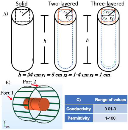
Fig. 1 A) Cylindrical structures used with size h = 24 cm, r1 = 5 cm, r2 = 1.5 - 4 cm and r3 = 1 cm, the region of interest is marked by the orange dashed line square. B) High pass birdcage coil at 128 MHz working frequency in green. Coil radius is 24 cm, the leg length is 20 cm and end ring width is 4 cm. Cylindrical structure placement in orange, middle lines show the extracted B1 maps. C) Range of values used.
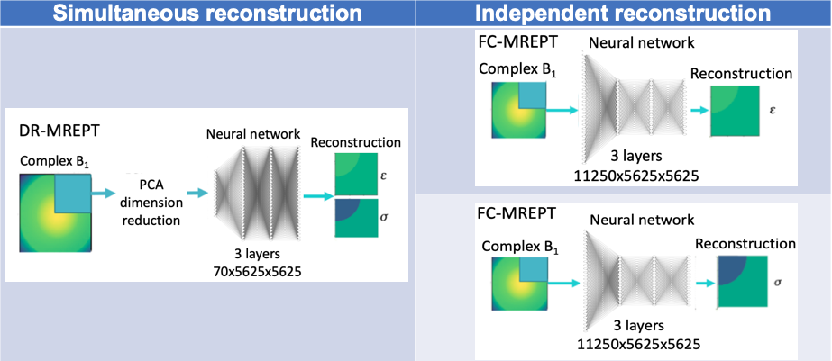
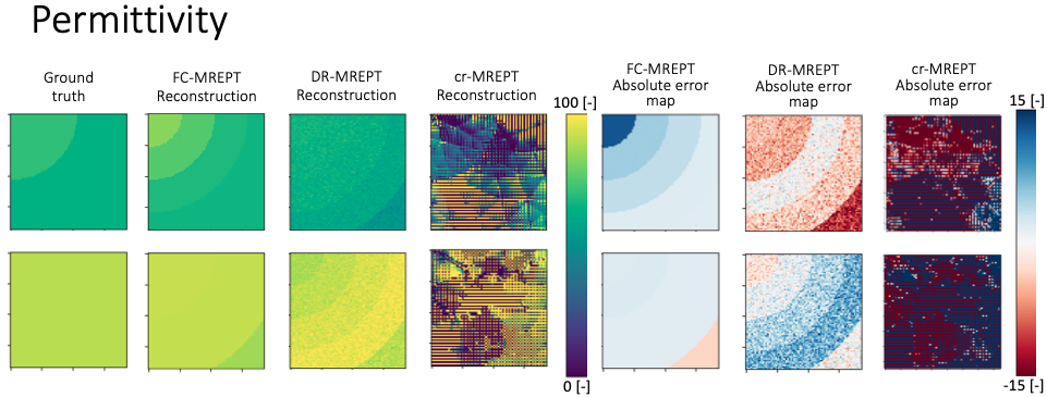
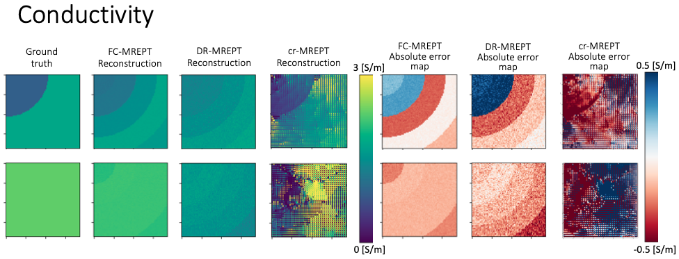
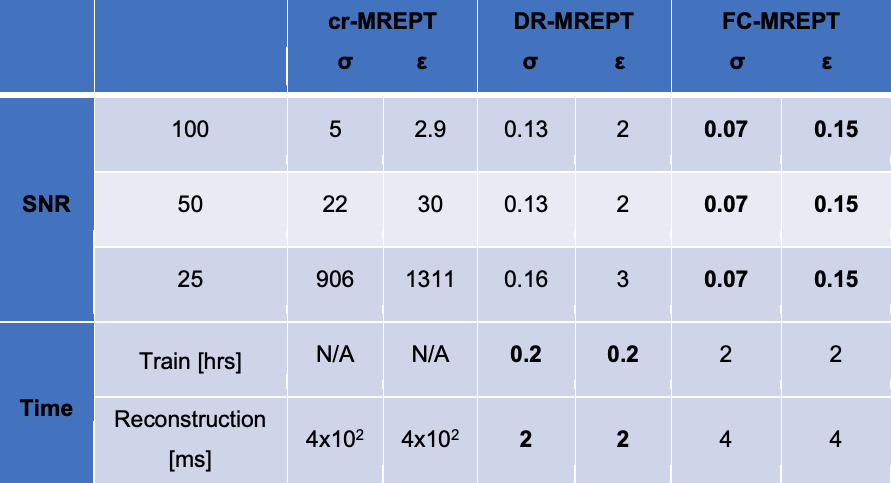
Fig. 5 Table of NRMSE reconstruction values for ML and analytical methods. The consistency of ML results, indicates noise robustness across the noise spectrum. Reconstruction time and training time for the ML and cr-MREPT model are also reported. FC-MREPT had the highest accuracy but was the slowest, DR-MREPT accuracy does not vary, but the training time is only one tenth, while reconstruction time is halved.