3179
Current Density Measurements in the Human Brain in-vivo during TES treatment, using Multi-Band methods1School of Biological and Health System Engineering, Arizona State University, Tempe, AZ, United States, 2Department of Radiology, Johns Hopkins University, Baltimore, MD, United States
Synopsis
Current density distribution measured in the brain can guide and verify electrical stimulation therapies. Recent studies have demonstrated current density images of human heads during TES using Magnetic Resonance Electrical Impedance Tomography (MREIT). Earlier MREIT approaches permitted imaging of three 5-mm-thick slices in a sequence lasting 6 minutes, a typical therapeutic TES administration time. MREIT sequences must be accelerated to obtain whole brain coverage. In this study, we demonstrate in-vivo use of multiband-accelerated multi-echo-gradient-echo MREIT acquisition methods to acquire 24 5-mm-thick slices over 6 minutes. Computed current density maps measured in the brain using both methods are compared.
Introduction
Refinement of neuromodulation techniques such as transcranial electrical stimulation (TES) includes focus on understanding mechanisms by which these techniques can affect attention, memory and other cognitive functions1. Until recently, measurement of the precise distribution of neuromodulation currents in-vivo has not been possible. However, studies have now demonstrated magnetic flux density and current density images of human heads using MREIT techniques2,3,4. In the studies of2,3, data were gathered from multiple human subjects undergoing transcranial AC stimulation-like procedures at frequencies of 10 Hz and 1.5 mA intensity. Three slices (thickness 5-mm) centered on electrode regions were acquired using the Philips mFFE sequence, in a time that depended linearly on the number of slices. However, more brain coverage is essential to perform group-level field-distribution analyses across subjects. We previously reported the performance of Multi-Band (MB) and SENSE acceleration applied to the mFFE sequence in gel phantoms5. In this study, we demonstrate in-vivo use of MB excitation pulses with the mFFE sequence6,7,8. We computed current density images using the local projected current density method9 and compared results against simulated current densities.Methods
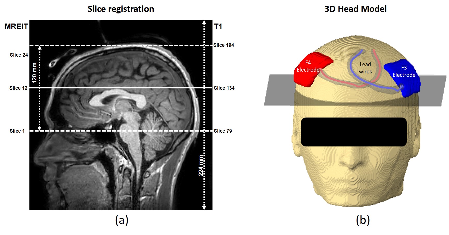
Magnetic flux density imaging experiment: All procedures were performed according to protocols approved by the Arizona State University Institutional Review Board. A neurologically normal volunteer was imaged using a 32-channel head coil in a 3T Philips Ingenia System during TES. A current intensity of 1.5mA with a frequency of ~10 Hz was applied to the subject’s head via surface electrodes (~36cm2) using F3-F4 montages, synchronized with the pulse sequence. T1-weighted structural images were collected using a 3D MPRAGE sequence with 224 mm (FH) x 224 mm (AP) x 224 mm (RL) field-of-view (FOV), and 1 mm isotropic resolution. The MB-mFFE MREIT dataset was acquired with an in-plane FOV of 224 mm (RL) x 896 mm (AP5) ), TR/TE= 50/7 ms, number of slices= 24, echoes= 10, echo spacing= 3 ms, acquisition matrix size=100 x 100, MB-factor=8, SENSE-factor=1, total scan time= 6 min. T1-weighted data was used to construct a computational model of the participant and track and correct for stray currents in electrodes and wires. Figure 1 shows the MREIT image locations and 3D numerical head model including electrodes (F3 and F4) and lead wire orientations. Multi-echo MREIT data was exported in PAR/REC format and processed offline with MATLAB 2018a (The MathWorks. Inc., Natick, MA, USA) to generate optimized magnetic flux density (Bz) maps2,3.Current density image reconstruction: We reconstructed the current density from experimentally measured Bz data ($$$B_z^m$$$). We used the projected current density10 measure, which is the best estimate of the three-dimensional current density from one component of magnetic flux density. Since the SNR in MR magnitude image within skin and skull regions were very low, standard deviations in Bz images were relatively high compared to those in brain tissues11. Inclusion of low SNR regions in reconstruction processing can distort reconstruction quality over the entire reconstruction region because the projected current density algorithm includes computation of the Laplacian of Bz data. Therefore, instead of reconstructing the current density images over the entire head, projected current density images $$$\mathbf{J}_R^P$$$ were only reconstructed using wire corrected Bz data ($$$B_z^{m,c}$$$) within a brain ROI9 as
$$\mathbf{J}_R^P=-\triangledown\alpha + (\frac{\partial \beta}{\partial y}, \frac{\partial \beta}{\partial x},0)$$
where $$$\begin{cases}\triangledown^{2}\alpha = 0\ \ \ \ \ \ \ \ \ in \ \Omega \\-\triangledown\alpha.n =g \ \ \ \ on \ \partial\Omega\end{cases}$$$ and $$$\begin{cases}\triangledown^{2}\beta = \frac{1}{\mu_{0}}\triangledown^{2}B_z^{m,c} \ \ \ \ \ \ \ \ in \ \Omega_{t}\\\beta = \frac{1}{\mu_{0}}(B_z^{m,c}-B_z^0) \ \ \ \ on \ \partial\Omega_{t} \end{cases}$$$ (1)
In (1), we describe the computation of the Laplacian of measured data. However, due to the boundary condition, artifacts from the wire stray magnetic field must be removed before computation. In this study, we implemented this using the stray magnetic field correction method12 developed by our group. We also computed the true current density ( $$$\mathbf{J}^{sim}|_R $$$) using FEM simulation for comparisons13.
Results and Discussion
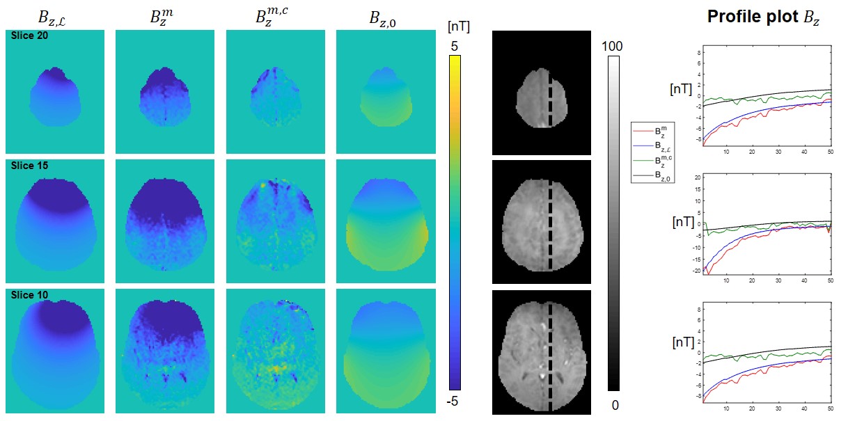
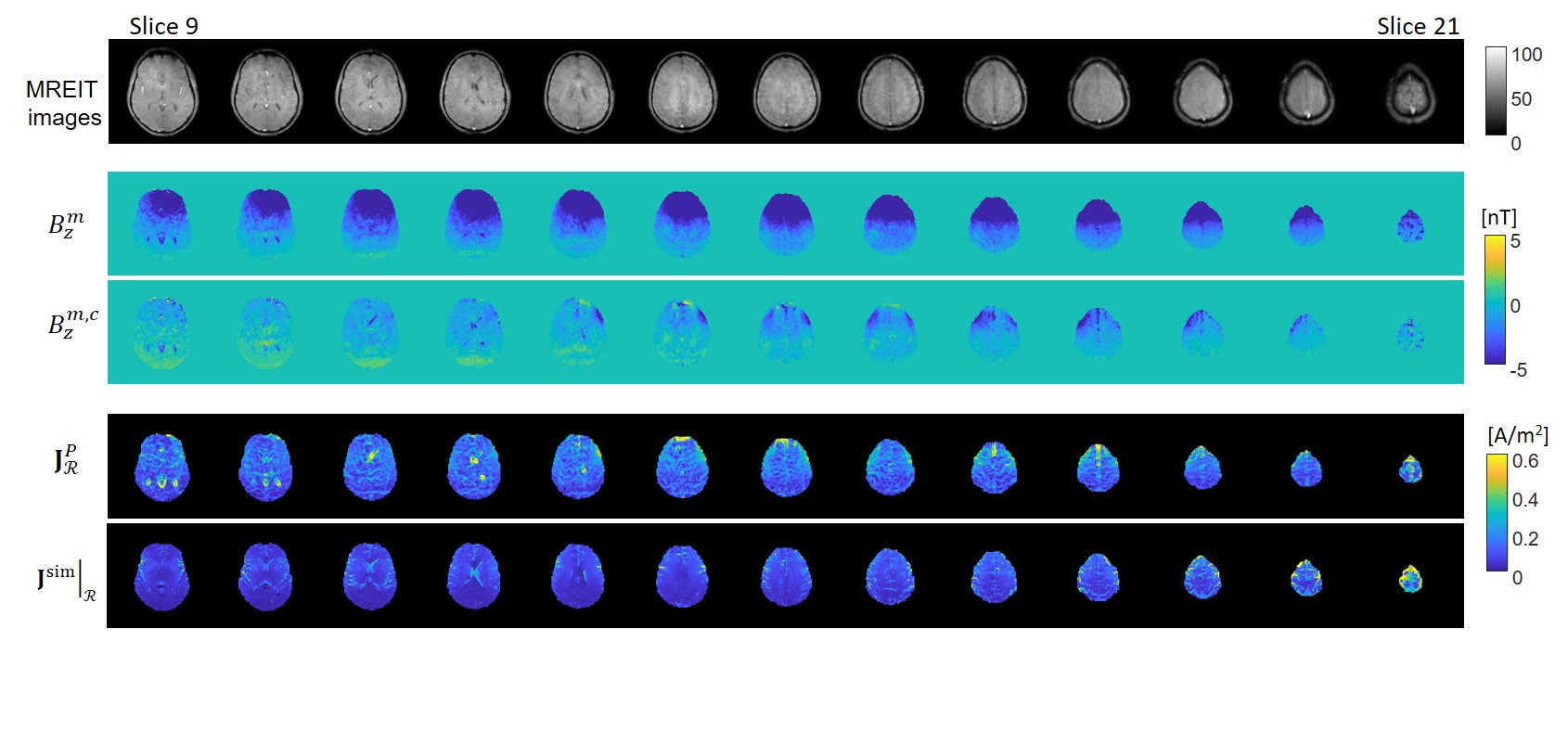
Figure 2 shows factors computed to correct for stray magnetic fields induced by lead wires, including simulated wire induced stray field ($$$B_{z,L}$$$ ), measured Bz ($$$B_z^m$$$ ), stray-field-corrected Bz ( $$$B_z^{m,c}$$$ ), uniform domain Bz ($$$B_{z}^0$$$ ), profile plot locations and Bz profile plots for slices 10, 20 and 15. Figure 3 shows the projected current density calculated for the measured data ($$$\mathbf{J}_R^P$$$ ) and the true current density ($$$\mathbf{J}^{sim}|_R $$$ ) obtained using the isotropic head computational model (slices 9-21).Conclusion
Calculated in-vivo current density maps were consistent with simulated data. Current density magnitudes in superior slices were larger than those in inferior slices, as expected (Fig. 3) because of the electrode montage (F3-F4) chosen for this study. Due to the low SNR of the Bz signal in inferior brain slices, we were not able to reconstruct the projected current density information from those slices (slices 1-8). Efficient denoising methods such as ramp-preserving denoising14 may improve the quality of Bz data, and hence projected current density reconstruction results.Acknowledgements
We gratefully acknowledge the assistance of Dr. Peter Boernert, Ulrich Katscher and Kay Nehrke (Philips Research, Hamburg) in providing access to sequences used in this study. The research reported in this abstract was supported by NIH award RF1MH114290 to RJS.References
1. Krause V, Meier A, Dinkelbach L, Pollok B. Beta Band Transcranial Alternating (tACS) and Direct Current Stimulation (tDCS) Applied After Initial Learning Facilitate Retrieval of a Motor Sequence. Front Behav Neurosci 2016;10:4.
2. Kasinadhuni AK, Indahlastari A, Chauhan M, et al. Imaging of current flow in the human head during transcranial electrical therapy. Brain Stimul 2017;10(4):764-772.
3. Chauhan M, Indahlastari A, Kasinadhuni AK, Schär M, Mareci TH, Sadleir RJ. Low-Frequency Conductivity Tensor Imaging of the Human Head in vivo using DT-MREIT: First Study. IEEE Transactions on Medical Imaging 2017;37(4):966-976.
4. Göksu C, Hanson LG, Siebner HR, Ehses P, Scheffler K, Thielscher A. Human in-vivo brain magnetic resonance current density imaging (MRCDI). NeuroImage2018;171: 26-39.
5. Chauhan M, Schär M , Sahu S, Mareci T H, and Sadleir R J Fast MREIT acquisition using Multi-Band and SENSE Techniques Proc. Intl. Soc. Mag. Reson. Med. 27 (2019) 5046.
6. Pruessmann KP, Weiger M, Scheidegger MB, Boesiger P. SENSE: sensitivity encoding for fast MRI. Magn Reson Med 1999; 42: 952– 962.
7. Breuer FA, Blaimer M, Heidemann RM, Mueller MF. Griswold MA, Jakob PM Controlled aliasing in parallel imaging results in higher acceleration (CAIPIRINHA) for multi-slice imaging. Magn Reson Med 2005;53: 684-691
8. Larkman D J, Hajnal J V, Herlihy A H, Coutts G A and Young I R 2001 Use of multicoil arrays for separation of signal from multiple slices simultaneously excited. J. Magn. Res. Imag. 13 313–7
9. Sajib S Z K, Kim H J and Kwon O I et al. Regional absolute conductivity reconstruction using projected current density in MREIT. Phys. Med. Biol. 2012; 57 (18):5841-59.
10. Park C, Lee BI, Kwon OI. Analysis of recoverable current from one component of magnetic flux density in MREIT and MRCDI. Phys Med Biol 2007;52(11):3001-3013.
11. Sadleir RJ, Grant S, Zhang SU, et al. Noise analysis in magnetic resonance electrical impedance tomography at 3 and 11T field strengths. Physiol Meas 2005; 26: 875– 884.
12. Sajib S Z K, Chauhan M and Banan G et al. Compensation of lead-wire magnetic field contributions in MREIT experiment using image segmentation: a phantom study. In Proc. Int. Soc. Magn. Reson. Med. 2019; 5049.
13. Huang, Y. et al. Automated MRI segmentation for individualized modeling of current flow in the human head.2013 J. Neural. Eng. 10 066004.
14. Lee CO, Jeon K, Ahn S, Kim HJ, Woo EJ Ramp-preserving denoising for conductivity image reconstruction in magnetic resonance electrical impedance tomography IEEE Trans Biomed Eng. 2011 58(7):2038-50.
Figures