3163
Simulating the effect of axonal dispersion and noise on anisotropic R2* relaxometry in white matter
Francisco Javier Fritz1, Luke J. Edwards2, Tobias Streubel1,2, Kerrin J. Pine2, Nikolaus Weiskopf2, and Siawoosh Mohammadi1,2
1Institute of System Neuroscience, Universitätklinikum Hamburg-Eppendorf, Hamburg, Germany, 2Department of Neurophysics, Max Planck Institute for Human Cognitive and Brain Sciences, Leipzig, Germany
1Institute of System Neuroscience, Universitätklinikum Hamburg-Eppendorf, Hamburg, Germany, 2Department of Neurophysics, Max Planck Institute for Human Cognitive and Brain Sciences, Leipzig, Germany
Synopsis
We introduced a forward model to simulate the effect of fibre dispersion on the angle-dependent GRE signal decay in different SNR conditions. We compared the classical signal model against three variations of the signal model derived from a second-order Taylor expansion in time of Wharton and Bowtell’s HCFM model, including a new model that accounts for fibre dispersion. We found a noise enhancement in the model parameters when using the second-order models. Moreover, we found that the orientation dependency of the GRE signal diminished for high dispersions.
Introduction
Quantitative MRI (qMRI) allows the characterisation of the biological structures in the human brain6. For example, apparent transverse R2*-weighted gradient-echo (GRE) MR images have been shown to be sensitive to both brain microstructure (e.g. fibres's myelination4) and the mean angular orientation (θμ) of fibre pathways relative to the main magnetic field, B08,9. We recently introduced an inverse model that allows separation of the orientation-independent part of R2* and an orientation-dependent higher-order term from a single multi-echo GRE measurement5. That model was based on the biophysical hollow cylinder fibre model (HCFM)8 assuming fully parallel fibres. Here we propose an extension of our model5 which heuristically includes the effect of fibre dispersion in the R2* estimation. To investigate the effects of dispersion on the GRE signal and the performance of the signal models, simulations were performed by combining the ensemble-averaged signal (EAS) model from the HCFM with angular fibre dispersion modelled by the Watson distribution2.Methods
Forward model: To study the effect of dispersion on the (R2*) signal decay, an EAS with dispersedly oriented cylinders (defined by κ, Fig.1B) around θμ with respect to B0 was simulated. In this experiment, we considered the idealized scenario7 where the myelin water compartment was neglected (SM≈0, R2*≈0), i.e. the simulated signal came from 1500 cylinders with intra-(SA) and extra-(SE) axonal compartments (Fig.1A). The averaged complex signal was sampled 5000 times with additive Gaussian complex noise to achieve a signal-to-noise ratio (SNR) of 100 (similar experimental SNR5) and infinity (ground truth)3. Simulation sampling scheme: θμ:[1:1:90]°, κ:[0.001:1.0:20,30:10:100,1e8 (perfectly parallel)] and echo time (TE):[0:0.1:40]ms.Inverse model and experimental conditions: Ten time-points evenly selected between 3-36 ms from simulated data were chosen to replicate experimental conditions5 and fulfil the static dephasing regime8. These signals were then fitted to 4 different models $$$m={M1,M2,M3,M4}$$$ of the form:
$$ln(|S_{WB}|)\approx\beta_0^m+\beta_1^mTE+\alpha_2^m{TE}^2$$
where $$$\alpha_2^m$$$ is defined as follows: $$$\alpha_2^{M1}=0$$$ (classical model, model 1), $$$\alpha_2^{M2}=\beta_2^{M2}$$$ is dependent on $$$\theta$$$ (model 2), $$$\alpha_2^{M3}(\theta)=\beta_2^{M3}\sin(\theta)^4$$$ (model 3) and $$$\alpha_2^{M4}(\theta)=\beta_2^{M4} <sin(\theta)^4>_{\theta^\prime,\kappa}$$$ (model 4). For the latter expression, the averaging of the angular component was performed using the Watson distribution, giving:
$$<\sin(\theta)^4>_{\theta',\kappa}=<1-2\cos(\theta)^2+\cos(\theta)^4>_{\theta',\kappa}$$
$$=(1-2\tau+\gamma)-(1+6\tau-5\gamma)\sin(\theta_\mu)^2+(3/8+35\gamma/8-15\tau/4)\sin(\theta_\mu)^4$$
$$\tau(\kappa)=\frac{2\kappa\exp(\kappa)-\sqrt{\pi\kappa}Erfi(\sqrt{\kappa})}{2\sqrt{\pi\kappa^3}Erfi(\sqrt{\kappa})},\gamma(\kappa)=\frac{3\sqrt{\pi}Erfi(\sqrt{\kappa}) + 2\sqrt{\kappa}\exp(\kappa)(2\kappa-3)}{4\sqrt{\pi}\kappa^2Erfi(\sqrt{\kappa})};Erfi(\sqrt{\kappa})=\frac{2}{\sqrt{\kappa}}\int_0^\sqrt{\kappa}exp(t^2)dt$$
where κ is the dispersion parameter and θμ is the angle between $$$\vec{B_0}$$$ and the mean orientation of the Watson distribution $$$\vec{\mu}$$$ (Fig.1B). The fitting of the model parameters, by given κ-θμ, was performed by linear regression and stabilised with a zeroth-order Tikhonov regularization for model 3-4 (of the form of λcos(θ)4 by targetting only the second-order component of the signal model). To estimate the optimal regularization parameter λ0 for SNR=100, we minimized the difference between model parameters at SNR=∞ and estimated parameters for a range of λ=1e-4:1e-4:1e-1 (λ0 of 0.01,0.02 for model 3-4, respectively). To compare the effect of SNR in the estimation of the model parameters for each model at different κ-θμ, the coefficient of variation (CV) of the estimated β’s across 5000 noise configurations were calculated.
Results and discussion
The simulated GRE signals in the case of dispersion are presented in Fig.2. The signal decay lost its angular dependency for large dispersion factors (solid lines for κ≈0) whereas it resembled the ideal case of parallel cylinders (dashed lines) for low dispersion factors (solid lines for κ>20). The parameters of model 1-2 behaved as previously reported5, demonstrating that the orientation dependence of β1M1 is transferred to β2M2 (Fig.3A,B). β2M3 values, at higher angles, were similar to β2M2, but for smaller angles (between 15°-30°) the differences increased exponentially; this divergence was down-weighted by the regularization leading to convergence towards zero (Fig.3C). For β2M4, the exponential increase for low angles for β2M3 was compensated, showing stable values for all the angles >20° (Fig.3D). The resulting estimation of the β parameters for all the models for the experimental SNR=100 is shown in Fig.4. β1M2, M3 and M4 showed a 5x increase in comparison to β1M1. In addition, β2M3 and M4 became greatly sensitive to noise for angles <45° across all κ (CV>1, see Table 1). Nevertheless, there was no bias introduced in the mean estimation of all the parameters in all the models, i.e. the estimated β’s are close to the ground truth (SNR=∞, Fig.3).Conclusion
In this work, we introduced a forward model to simulate the effect of fibre dispersion on the angle-dependent GRE signal decay in different SNR conditions. Moreover, we proposed a new inverse model that accounts for this effect on the estimated parameters and compared it with published models5 for an experimentally-relevant SNR regime. We found noise enhancement in the estimated parameters of the second-order models (M2,M3,M4) as compared to M1, which can be explained by the increased condition number in the inverse model1 when introducing the second-order decay parameter β2. Interestingly, we found for β2 noise enhancement for highly aligned fibres for angles <45°, which might be explained by the vanishing quadratic signal-contribution for low angles. Nevertheless, models 1-2 proved to be still valid even for moderate dispersion. Future work will assess the errors made by neglecting the myelin compartment and the position dependence of the frequency offsets, as already simulated10.Acknowledgements
This work was supported by the German Research Foundation (DFG Priority Program 2041 "Computational Connectomics”, [AL 1156/2-1;GE 2967/1-1; MO 2397/5-1; MO 2249/3–1], by the Emmy Noether Stipend: MO 2397/4-1) and by the BMBF (01EW1711A and B) in the framework of ERA-NET NEURON and the Forschungszentrums Medizintechnik Hamburg (fmthh; grant 01fmthh2017). The research leading to these results has received funding from the European Research Council under the European Union's Seventh Framework Programme (FP7/2007-2013) / ERC grant agreement n° 616905.References
- Aster, R.C., Borchers, B., Thurber, C.H., 2019. Appendix A - Review of Linear Algebra, in: Aster, R.C., Borchers, B., Thurber, C.H. (Eds.), Parameter Estimation and Inverse Problems (Third Edition). Elsevier, pp. 309–340.
- Fisher, N.I., Lewis, T., Embleton, B.J.J., 1993. Statistical Analysis of Spherical Data. Cambridge University Press.
- Gudbjartsson, H., Patz, S., 1995. The rician distribution of noisy mri data. Magn. Reson. Med. 34, 910–914
- Li, T.-Q., Li, T.-Q., Yao, B., van Gelderen, P., Merkle, H., Dodd, S., Talagala, L., Koretsky, A.P., Duyn, J., 2009. Characterization of T(2)* heterogeneity in human brain white matter. Magn. Reson. Med. 62, 1652—1657.
- Papazoglou, S., Streubel, T., Ashtarayeh, M., Pine, K.J., Edwards, L.J., Brammerloh, M., Kirilina, E., Morawski, M., Jäger, C., Geyer, S., Callaghan, M.F., Weiskopf, N., Mohammadi, S., 2019. Biophysically motivated efficient estimation of the spatially isotropic component from a single gradient-recalled echo measurement. Magn. Reson. Med. 82, 1804–1811.
- Tofts, P.S., 2004. Concepts: Measurement and MR, in: Quantitative MRI of the Brain. John Wiley & Sons, Ltd, pp. 1–15.
- Wharton, S., Bowtell, R., 2013. Gradient Echo Based Fiber Orientation Mapping using R2* and Frequency Difference Measurements. NeuroImage 83
- Wharton, S., Bowtell, R., 2012. Fiber orientation-dependent white matter contrast in gradient echo MRI. Proc. Natl. Acad. Sci. 109, 18559.
- Wiggins, C., Gudmundsdottir, V., Bihan, D., Lebon, V., Chaumeil, M., 2008. Orientation Dependence of White Matter T 2 * Contrast at 7 T : A Direct Demonstration. Proc. 16th Annu. Meet. ISMRM Tor. Can.
- Xu, T., Foxley, S., Kleinnijenhuis, M., Chen, W.C., Miller, K.L., 2018. The effect of realistic geometries on the susceptibility-weighted MR signal in white matter. Magn. Reson. Med. 79, 489–500
Figures
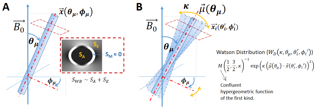
Figure 1: Wharton and Bowtell (WB) model (A) and extension to account dispersion (B)
used for simulation. (A) The WB signal approximation neglects the
myelin water compartment (SM≈0), describing the ensemble-averaged
signal (EAS) contribution from extra-(SE) and intra-(SA)
axonal compartments for one cylinder ($$$\vec{x_\mu}$$$) with orientation
(θμ,φμ) with respect to B0. (B)
EAS contribution of an ensemble of N=1500 cylinders ($$$\vec{x_i}$$$ (θi,φi))
following the Watson distribution with dispersion factor κ
with respect the averaged-orientation $$$\vec{\mu}$$$.
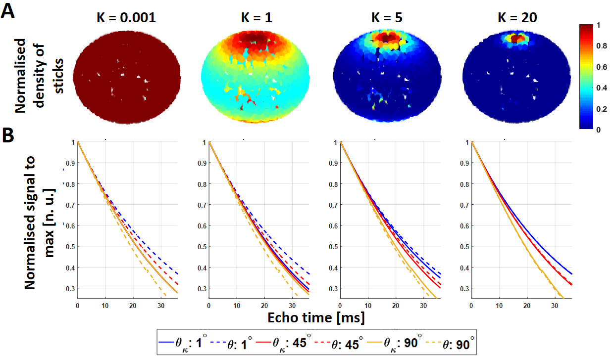
Figure 2: Dispersion
effect in R2* signal decay: (A) The weights from the Watson distribution as a
function of κ can
be represented as the normalised density of sticks across the sphere. (B)
Corresponding signal decay (solid lines) for each κ value at three main orientation angles with respect
to B0 (θμ): 1°, 45° and 90° compared with the perfectly
parallel cylinders (κ = 1e8,
dashed lines). At increasing κ, the signal decay becomes sensitive
to θμ, as expected.
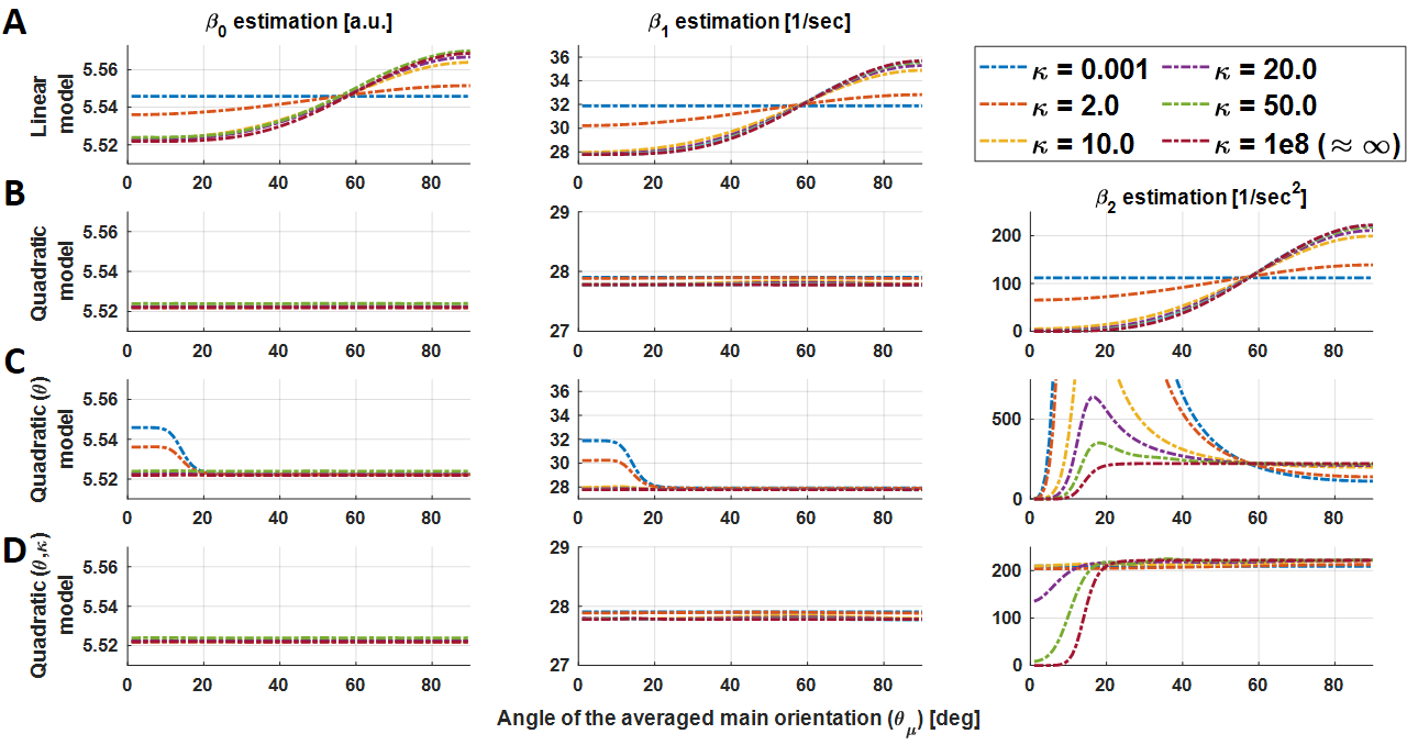
Figure 3: Parameter
estimation (β’s, columns) for all the models (rows) at different
dispersion factors for the ground truth condition (SNR = ∞). For the first
model (A), from low κ values, the parameters become visible dependent on θμ. This dependency is corrected by β2 in
more complex models (B, C and D). The proposed model (4th row) is
capable of predicting the dispersion component for moderate angles (above 20°).
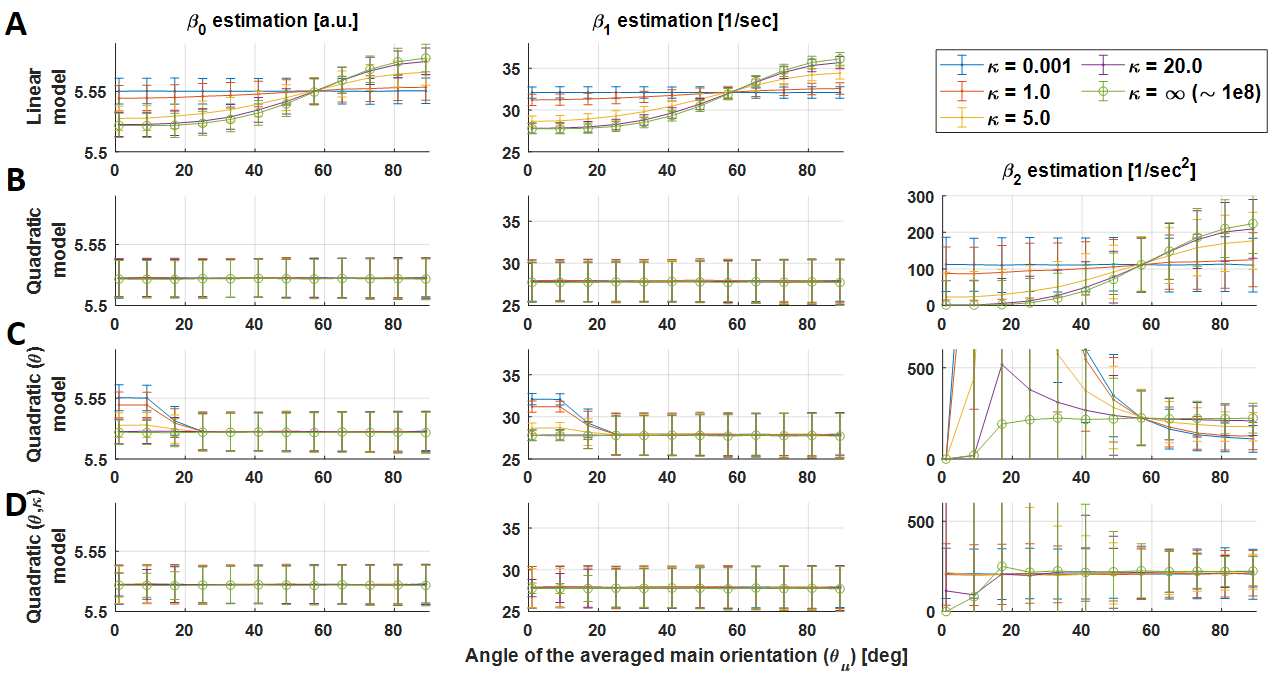
Figure 4: Parameter
estimation β0, β1 and β2 (columns) for
all the models (rows) at different dispersion factors for the experimental
SNR condition (SNR = 100). Qualitatively, the parameter estimation behaves similarly
to in the ground truth condition. However, variation in β2 estimation is
exacerbated for low θμ
angles (see Table 1).
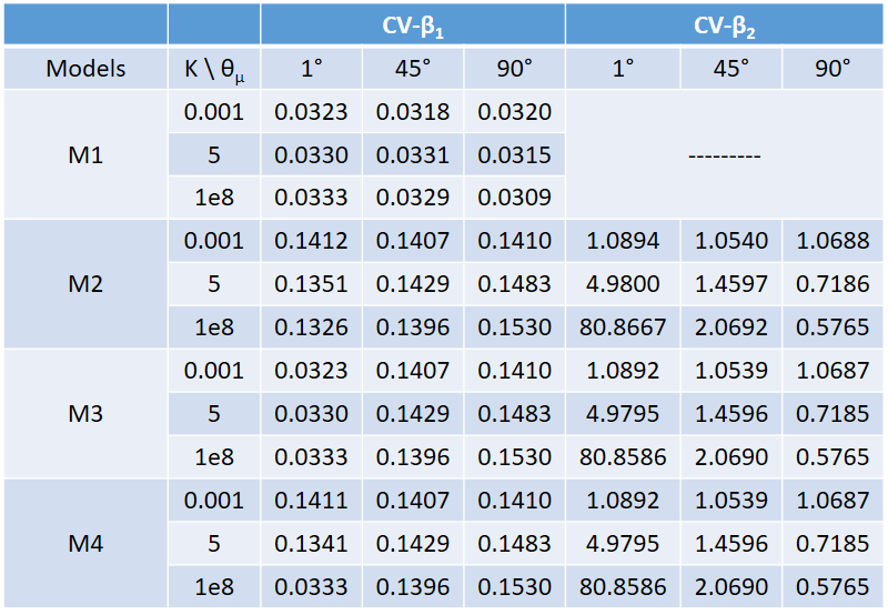
Table 1: Coefficient
of variation (CV) for β1 and β2
estimated at SNR = 100 for all the models. Three angles (1°, 45° and 90°) and
three dispersion values (0.001, 5 and 1e8 or fully parallel) were selected.
From those values, reduced CVs are achieved for β1M1 in
the small angles regime, whereas for β2 values are the highest (along with all models).