Introduction

The macromolecular proton fraction ($$$f$$$ = MPF) is a quantitative parameter calculated from magnetization transfer (MT) images which describes the proportion of signal arising from protons in water bound to macromolecules relative to free water, and has been used to characterize myelin structure and content in the brain. The single point MT experiment quantifies $$$f$$$ from two spoiled, gradient echo images: an MT-weighted and MT reference image ($$$MT_∆$$$ and $$$MT_0$$$, respectively). After several approximations, an analytic solution for the observed MT-weighted signal ($$$MT_∆$$$) as a function of tissue and sequence parameters has been derived [1] in Eq. 1: $$ Mz = (1-f)\frac{A + R1_F{\cdot}s{\cdot}W}{A + (R1_F + k){\cdot}s{\cdot}W - (R1_B + k(1-f)/f + s{\cdot}W){\cdot}log(cos\alpha{\cdot})/Tr}$$ where $$$R1_F$$$ and $$$R1_B$$$ are the relaxation rate constants of the free and bound pools, $$$A = R1_F{\cdot}R1_B + R1_F{\cdot}R + R1_B{\cdot}R{\cdot}f/(1-f)$$$, $$$W$$$ is the saturation rate for the bound pool [2], α is the excitation flip angle, and $$$s$$$ is the saturation pulse width divided by TR. For the single-point method, $$$M = MT_∆/MT_0$$$ is modelled and the tissue parameters characterizing the exchange and relaxation rates of the bound pool are fixed, such that $$$W$$$ becomes a constant and the only remaining unknown in the equation is $$$f$$$ if separate measurements are made of R1_obs = 1/T1, B1 and B0 maps. This nonlinear function of $$$f$$$ requires a solver to be called for every voxel in order to calculate the MPF maps, which is prohibitively time consuming for large 3D data sets. This can be sped up by interpolating a lookup table predefined for a single set of sequence parameters and a range of possible T1, B1, B0 and M values, but still requires a voxel-wise computation.

In this work, the equation for the normalized signal, $$$M$$$, has been inverted to provide an analytic solution for MPF. This allows forward computation of MPF maps via matrix operations, resulting in a drastic reduction in processing time.

Methods

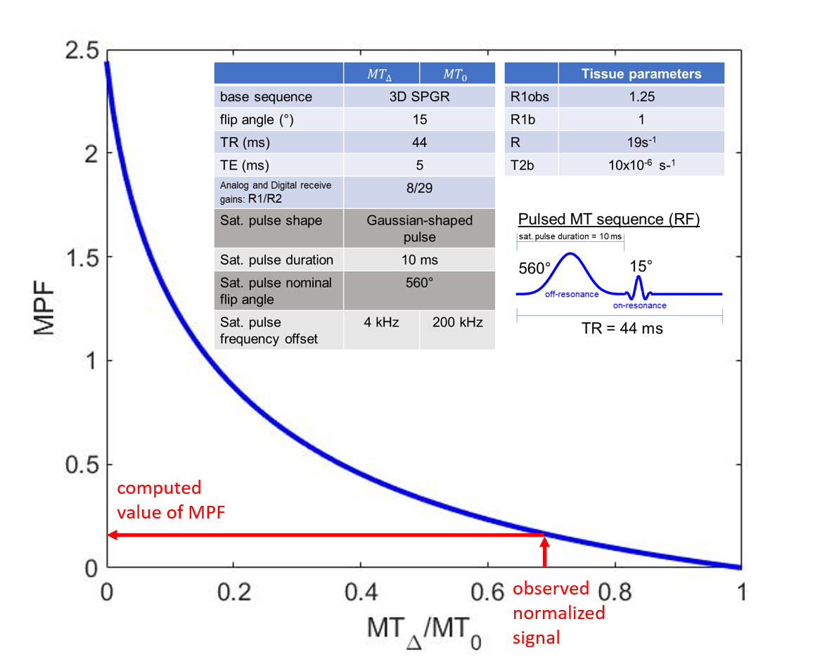
The normalized signal is modelled as: $$$M = MT_∆/MT_0$$$ where $$$MT_∆$$$is as in Eq.1 and $$$MT_0$$$ has no saturation (W = 0). Fig 1 shows a plot of simulated MPF vs $$$M$$$. If a substitution of variables is made ($$$x = f/(1-f))$$$, $$$M$$$ becomes a rational expression in $$$x$$$ of degree 2. The equation is rearranged as follows: $$MT_∆(x) – MT_0 (x)*M=0$$ and $$$x$$$ can be obtained by using the observed value of $$$M$$$ and solving for the zeros using the quadratic formula, i.e. Eq. 2: $$x=\frac{-b\pm\sqrt{b^2-4ac}}{2a}$$ where, a, b and c are constants which can be computed from fixed or measured parameters. The negative root is discarded because the value of $$$f$$$ is strictly greater than 0 ($$$x$$$ is always positive).

Fig. 2 shows the algebraic expressions for a,b and c under the assumption that R1_B is fixed and R1_F is written in terms of R1_obs: $$R1_F=R1_{obs}-(f*R(R1_B-R1_{obs}))/(1-f)(R1_B-R1_{obs}+R)$$
Fig. 3 shows the algebraic expressions for a, b and c under the simplification that the relaxation constants of the two pools are equal: $$R1_F= R1_B = R1_{obs}$$ After solving for $$$x$$$, $$$f$$$ is computed by $$$f = x/(1+x)$$$ (Eq. 3)

MT-weighted and MT-reference images were acquired (matrix 256x160x122) in human brain using a spoiled gradient echo sequence with the addition of a saturation pulse for MT contrast, along with T1 and B1 maps (no B0 correction for this example). Sequence details are in Fig. 1. We compared two methods of computing MPF from this data: 1) voxelwise interpolation of a lookup table 2) direct calculation from Eq.3.

Results

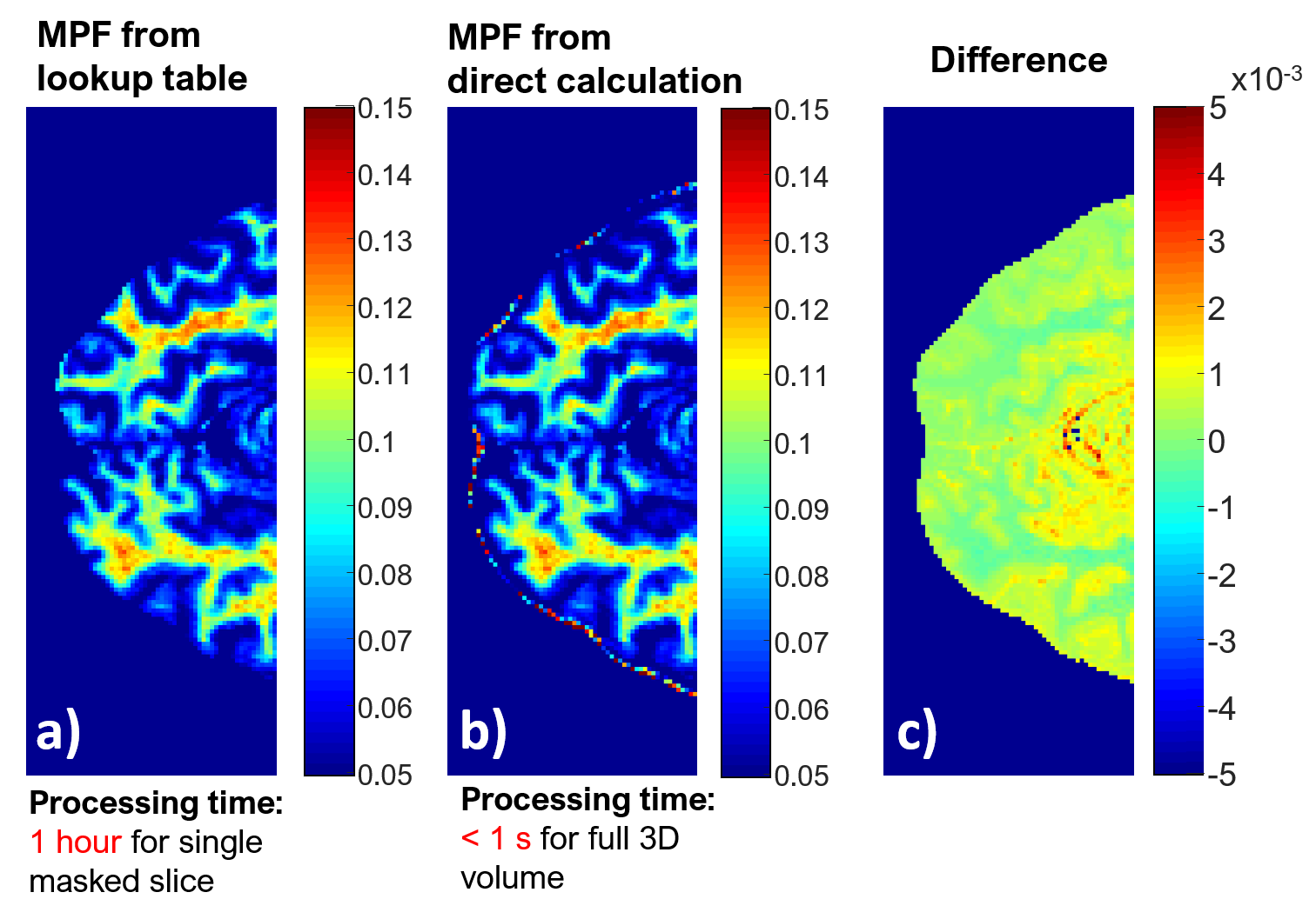
Fig.4a) is the resulting MPF from the lookup table interpolation (Processing time: 1 hr for one masked slice (256x160)) and b) from the direct computation using the method with R1_B = 1s^-1 (Processing time: <1s for entire volume (256x160x122). The differences (mean difference being (4.3±4.8) x10-4 in the images c) are below the order of the precision of the lookup table interpolation, which sampled $$$M = MT_∆/MT_0$$$ in increments of 0.02.

Discussion

Inverting the signal equation to obtain an analytic expression for MPF allows rapid computation of MPF maps from direct matrix operations, removing the need for solvers or lookup tables which need to be generated anew for any change in sequence parameters. The non-zero mean difference between the lookup table linear interpolation and the forward calculation is due to the positive concavity of the function of MPF vs $$$M$$$. Every point of the function on a line drawn between two computed points will be greater than the original function. Although the approximation for MPF using equal longitudinal rate constants yields similar results when R1_B is fixed at 1 and R1_F is computed from R1_obs, it has been suggested that the true value of R1_B is much shorter [3] and the first method, although with longer expressions for the constant coefficients, allows R1_B to be set to any constant that is desired.

Conclusion

The analytic expression derived in this work allows for rapid measurement of 3D MPF maps from data acquired in the single point MT experiment. This will also accelerate optimization strategies which previously required many runs of a solver algorithm and can now directly compute MPF.

Acknowledgements

The author would like to acknowledge Sofia Chavez for helpful discussions.