3130
pH mapping of brain tissue by a deep neural network trained on 9.4T CEST MRI data – pH-deepCEST1High-field Magnetic Resonance Center, Max Planck Institute for Biological Cybernetics, Tuebingen, Germany, 2Department of Biomedical Magnetic Resonance, Eberhard Karls University Tuebingen, Tuebingen, Germany, 3Department of Neuroradiology, University Hospital Erlangen, Erlangen, Germany
Synopsis
The pH value is of major importance for most physiological processes and may change due to altered metabolism in pathologies. In the present work, we exploit the inherent dependency of CEST MR data on pH with a new approach: train neural networks to map voxel-by-voxel from multi-B1+ CEST spectra to pH value. Measurements were performed in homogenate of pig brain tissue at 9.4T ultra high field. Prediction of absolute pH values was possible and predictions were stable against inhomogeneity in B1+. We hope this proof of concept might be a first small step towards high-resolution 3D pH maps in vivo.
Introduction
The pH value is of importance for nearly all physiological processes in vivo and it is often altered in pathologies due to altered metabolism – for example in tumors or in ischemic stroke. To be able to generate a 3D pH map with reasonable spatial resolution is thus of great interest in MRI. One way to access pH noninvasively in vivo with high precision is 31P MR spectroscopy (1). However, 31P MRS suffers from low signal and thus relatively poor spatial resolution. In 1H CEST MRI the pH value is an inherent property of all measured signals since it catalyzes the exchange rates (2) which can be exploited for pH mapping (3). Moreover, the signal of 1H CEST is much higher compared to 31P. However, at in vivo conditions the pH dependency of the CEST signal is rather complex and not easy to model. In the present work, we aim to extract the pH value from CEST data by training a neural network (NN) to predict pH values from multi-B1 CEST spectra acquired in post mortem pig brain at 9.4T as an in-vivo-like tissue sample.Methods
All measurements were performed at a 9.4T human whole body MR scanner (Siemens Healthineers, Erlangen, Germany) with a custom-built 18/32 Tx/Rx head coil (4) applying a 3D-GRE sequence (5) (TE/TR=1.91/3.76ms, FOV=147x120x40mm³, ROxPEx3D=96x78x8; 690Hz/pix; in PE: GRAPPA=2). CEST measurements were performed for 112 saturation offsets at three different nominal B1+ values (0.4, 0.6, 0.9 µT) with 150x15ms Gaussian pulses at DC=50% (recovery times/M0=5/12s). Four interleaved WASABI (6) measurements were added. Samples were prepared from fresh pig brain provided by the local slaughterhouse (no animals killed only for the purpose of this work). Vessels, brain stem and penumbra were removed before homogenate was produced. The pH value in the homogenate was adjusted using 1M NaOH and HCl and measured using a pH electrode (inoLab pH 720, WTW, Weilheim, Germany). A deep feed-forward neural network (NN), with probabilistic output layer for uncertainty quantification, was trained voxel-by-voxel on data sets that contained CEST spectra of three different B1+, and the absolute B1+ values obtained by WASABI. Target pH values for the NN were determined with the pH electrode for each sample. For testing the NN, additional samples with slightly different pH values compared to the training set were created and measured with the exact same MRI protocol.Results
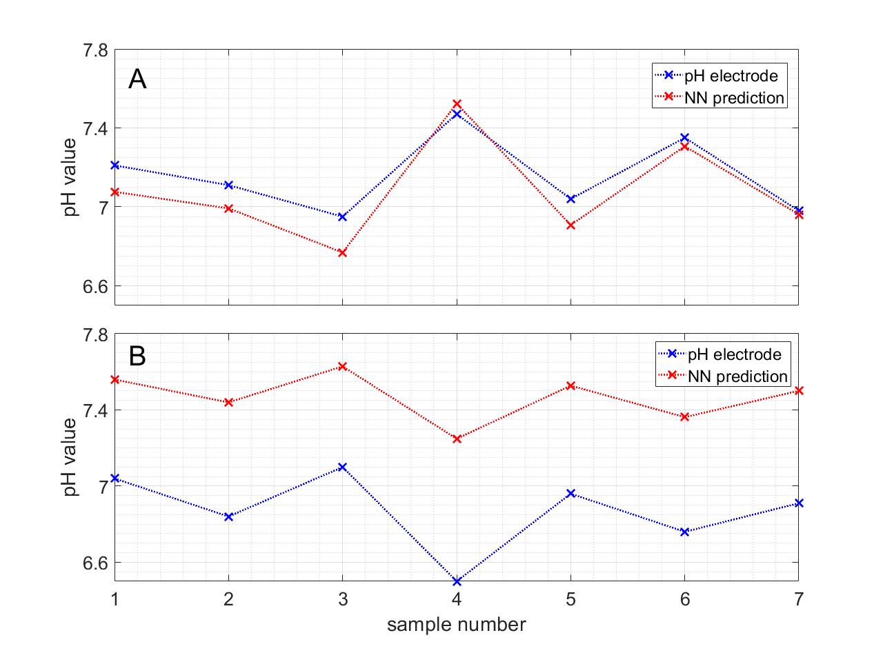
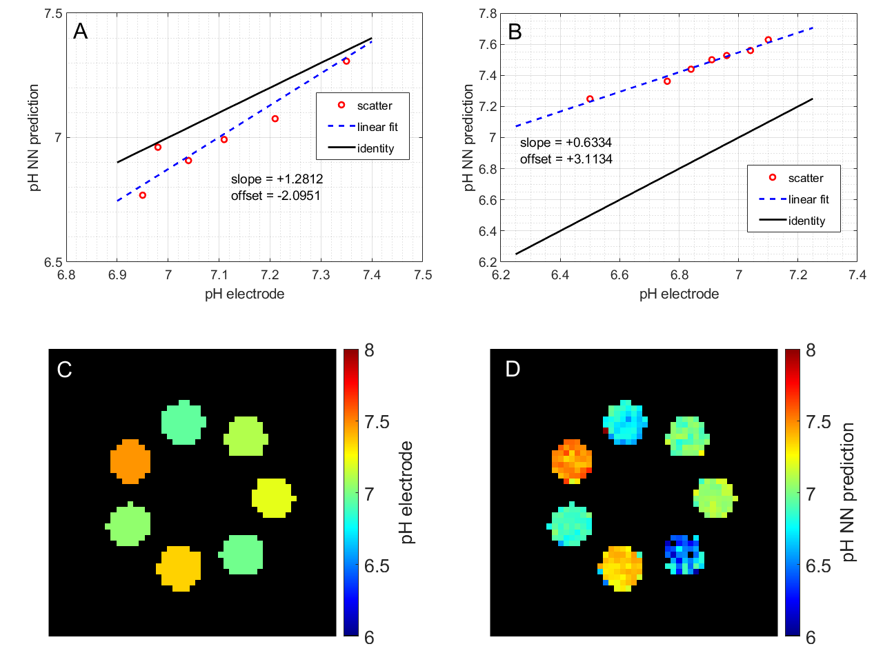
Investigation of different NN architectures showed that two layers with 100 neurons each were suitable for the given task with dropout rate during training set to 10%. The calibration mean squared error as suggested by Kendall et al. (7) was found to be below 5% for the optimized NN architecture. The NN was able to predict pH with an average deviation <0.1 pH (maximum deviation <0.2 pH) in phantoms that were not contained in the training set. In Figure 1A, the corresponding pH ground truth and NN prediction values are shown for seven samples. The predicted pH values match the ground truth well, as indicated by the slope (+1.2812; ideal: 1.0) shown in Figure 2A. The same network trained on 25°C data was also applied to additional test samples measured at 37°C. This increased the average prediction error by a factor of 2.4, however, the relative pH contrast between the samples was still predicted correctly (Figure 1B/2B). The spatial distribution of predicted pH values was homogeneous within single samples (Figure 2CD) and on average spatial std/mean was 8%. The B1+ values differed by 21% with the same metric. Figure 3 shows scatter plots and correlation coefficients for predict pH against measured relative B1+. Only weak correlation (in 5 of 7 cases significant with P<0.05) was seen with min/max/average correlation coefficients of -0.4991/0.3526/0.0031 for different samples. Thus, the NN is robust against B1+ inhomogeneity. Indeed the largest absolute correlation coefficient was observed for a sample that had a 2.2 times smaller T1 (≈840ms) as contained in training data (mean±std: (1872±27)ms).Discussion
The pH-deepCEST NN was able to predict pH values of unknown samples with high accuracy. Interestingly, the network also generalized to samples with different temperature as contained in the learning data set, and could predict pH differences accordingly; still the absolute pH value was biased. Nevertheless, other parameters such as T1, T2 and especially concentration were kept constant and their influence on the predictions must be further evaluated since they would spatially differ in vivo and alter CEST MRI spectra. For example, it was observed that T1 might introduce some bias. Still, being able to exploit 1H CEST MRI data to predict pH values would strongly increase spatial resolution as compared to spectroscopic imaging; in addition clinical translation of such a pH mapping might be simpler for a 1H-based MRI method.Conclusion
The derived results can be seen as proof of principle for the application of neural networks to predict absolute pH values based on 1H CEST MRI data of brain tissue.Acknowledgements
The financial support of the Max Planck Society, German Research Foundation (DFG, grant ZA 814/2-1), and European Union’s Horizon 2020 research and innovation programme (Grant Agreement No. 667510) is gratefully acknowledged.References
1. Moon RB, Richards JH. Determination of Intracellular pH by 31P Magnetic Resonance. J. Biol. Chem. 1973;248:7276–7278.
2. Englander SW, Downer NW, Teitelbaum H. Hydrogen Exchange. Annual Review of Biochemistry 1972;41:903–924 doi: 10.1146/annurev.bi.41.070172.004351.
3. Zhou J, Payen J-F, Wilson DA, Traystman RJ, van Zijl PCM. Using the amide proton signals of intracellular proteins and peptides to detect pH effects in MRI. Nature Medicine 2003;9:1085–1090 doi: 10.1038/nm907.
4. Avdievich NI, Giapitzakis I-A, Bause J, Shajan G, Scheffler K, Henning A. Double-row 18-loop transceive–32-loop receive tight-fit array provides for whole-brain coverage, high transmit performance, and SNR improvement near the brain center at 9.4T. Magnetic Resonance in Medicine 2019;81:3392–3405 doi: 10.1002/mrm.27602.
5. Zaiss M, Ehses P, Scheffler K. Snapshot‐CEST: Optimizing spiral‐centric‐reordered gradient echo acquisition for fast and robust 3D CEST MRI at 9.4 T. NMR in Biomedicine 2018;31 doi: 10.1002/nbm.3879.
6. Schuenke P, Windschuh J, Roeloffs V, Ladd ME, Bachert P, Zaiss M. Simultaneous mapping of water shift and B1 (WASABI)-Application to field-Inhomogeneity correction of CEST MRI data. Magn Reson Med 2017;77:571–580 doi: 10.1002/mrm.26133.
7. Kendall A, Gal Y. What Uncertainties Do We Need in Bayesian Deep Learning for Computer Vision? In: Guyon I, Luxburg UV, Bengio S, et al., editors. Advances in Neural Information Processing Systems 30. Curran Associates, Inc.; 2017. pp. 5574–5584.
Figures