3040

Deep Learning-based Fast Magnetic Resonance Spectroscopy

Xiaobo Qu¹, Yihui Huang¹, Hengfa Lu¹, Tianyu Qiu¹, Di Guo², Tatiana Agback³, Vladislav Orekhov⁴, and Zhong Chen¹
¹Department of Electronic Science, Xiamen University, Xiamen, China, ²School of Computer and Information Engineering, Xiamen University of Technology, Xiamen, China, ³Department of Molecular Sciences, Swedish University of Agricultural Sciences, Uppsala, Sweden, ⁴Department of Chemistry and Molecular Biology, University of Gothenburg, Gothenburg, Sweden

Synopsis

Nuclear magnetic resonance (NMR) spectroscopy serves as an indispensable tool in chemistry and biology but often suffers from long experimental time. In this work, we present a proof-of-concept of application of deep learning and neural network for high-quality, reliable, and very fast NMR spectra reconstruction from limited experimental data. Experimental results show that the neural network training can be achieved using solely synthetic NMR signal with exponential functions, which lifts the prohibiting demand for a large volume of realistic training data usually required in the deep learning approach.

Purpose

NMR spectroscopy is an invaluable biophysical tool in modern chemistry and life sciences, while the duration of NMR experiments increases rapidly with spectral resolution and dimensionality1. To accelerate data acquisition, several methods have been established to reconstruct high-quality spectra from Non-Uniform Sampling (NUS) data. However, different prior assumptions are applied in these methods and not well understood and the combination of the best features. Deep learning (DL) does not require any predefined formal priors, which retrieves the essential features from the amounts of realistic training data required in most cases. In this work, we demonstrate that successful training of the neural network in the DL is possible using solely synthetic data generated by exponential functions. Besides, the DL enables 10 times faster spectra reconstruction than conventional methods.

Methods

Our method solely uses the synthetic data as training data. The fully sampled FID x is simulated according to the classical exponential function modeling as^1-6: $${{x}_{n}}=\sum\limits_{j=1}^{J}{\left( {{A}_{j}}{{e}^{i{{\phi }_{j}}}} \right){{e}^{-\frac{n\Delta t}{{{\tau }_{j}}}}}{{e}^{in\Delta t2\pi {{\omega }_{j}}}}}, (1)$$where n is the n^th entry of the FID, J is the number of exponentials, A_j, ϕ_j, τ_j and ω_j are the amplitude, phase, decay time and frequency, respectively, of the j^th exponential, Δt denotes the time increment between two samples. The corresponding spectrum satisfies $$$\mathbf{s}=\mathbf{Fx}$$$, where $$$\mathbf{F}$$$ is the Fourier transform and $$$\mathbf{x}$$$ is the fully sampled FID, and the undersampled FID obeys $$$\mathbf{y}=\mathbf{Ux}$$$, where $$$\mathbf{U}$$$ is the undersampling operator.A flowchart of the proposed DL NMR is shown in Fig.1. The initial spectrum that inputs the neural network is computed as $$${{\mathbf{s}}_{\mathbf{U}}}={{\mathbf{F}}^{H}}{{\mathbf{U}}^{T}}\mathbf{y}$$$, where $$${{\mathbf{U}}^{T}}$$$is the adjoint operator of $$$\mathbf{U}$$$ and $$${{\mathbf{F}}^{H}}$$$ is the forward Fourier transform. This initial spectrum is with strong artifacts since those unsampled FID data are filled with zeros on non-acquired positions.The spectrum $$${{\mathbf{s}}_{\mathbf{U}}}$$$ is fed into the 8-layers densely connected convolutional neural networks, known as dense CNN⁷. This neural network learns a map $$${{f}_{CNN}}$$$ to reduce the spectrum artifact and yield the ‘clean’ spectrum denoted as $$${{\mathbf{\hat{s}}}_{CNN}}$$$.A data consistency module is incorporated to ensure reconstructed spectra are aligned to acquired data. Given the output of dense CNN $$${{\mathbf{\hat{s}}}_{CNN}}$$$, the spectrum is modified as$${{\mathbf{\hat{s}}}_{DC}}=\arg \underset{{{\mathbf{s}}_{DC}}}{\mathop{\min }}\,\left\{ {{\left\| {{\mathbf{s}}_{DC}}-{{{\mathbf{\hat{s}}}}_{CNN}} \right\|}^{2}}+\lambda {{\left\| \mathbf{y}-\mathbf{U}{{\mathbf{F}}^{T}}{{\mathbf{s}}_{DC}} \right\|}^{2}} \right\}, (2)$$ where $$$\left\| \cdot \right\|$$$ denotes the norm of a vector, $$${{\mathbf{F}}^{T}}$$$ the inverse Fourier transform, $$${{\mathbf{s}}_{DC}}$$$ the underlying spectrum to be optimized, and $$${{\mathbf{\hat{s}}}_{DC}}$$$is the output of data consistency module. A closed form solution of Eq. (2) is$${{\mathbf{\hat{s}}}_{DC}}=\mathbf{F}{{\left( \lambda {{\mathbf{U}}^{T}}\mathbf{U}+\mathbf{1} \right)}^{-1}}\left( \lambda {{\mathbf{U}}^{T}}\mathbf{y}+{{\mathbf{F}}^{T}}{{{\mathbf{\hat{s}}}}_{CNN}} \right), (3)$$ where $$$\mathbf{1}$$$ is an identity matrix and $$${{\left( \cdot \right)}^{-1}}$$$ denotes the inverse of a matrix. In our implementation, the regularization parameter $$$\lambda $$$ balances data consistency between the acquired data points in the initial data $$$\mathbf{y}$$$ and the predicted data point obtained with the dense CNN, which equal to $$${{10}^{6}}$$$ and works well for all the tested spectra. The overall loss function in our implementation is mean square error between output of the data consistency module and fully sampled spectrum.

Results

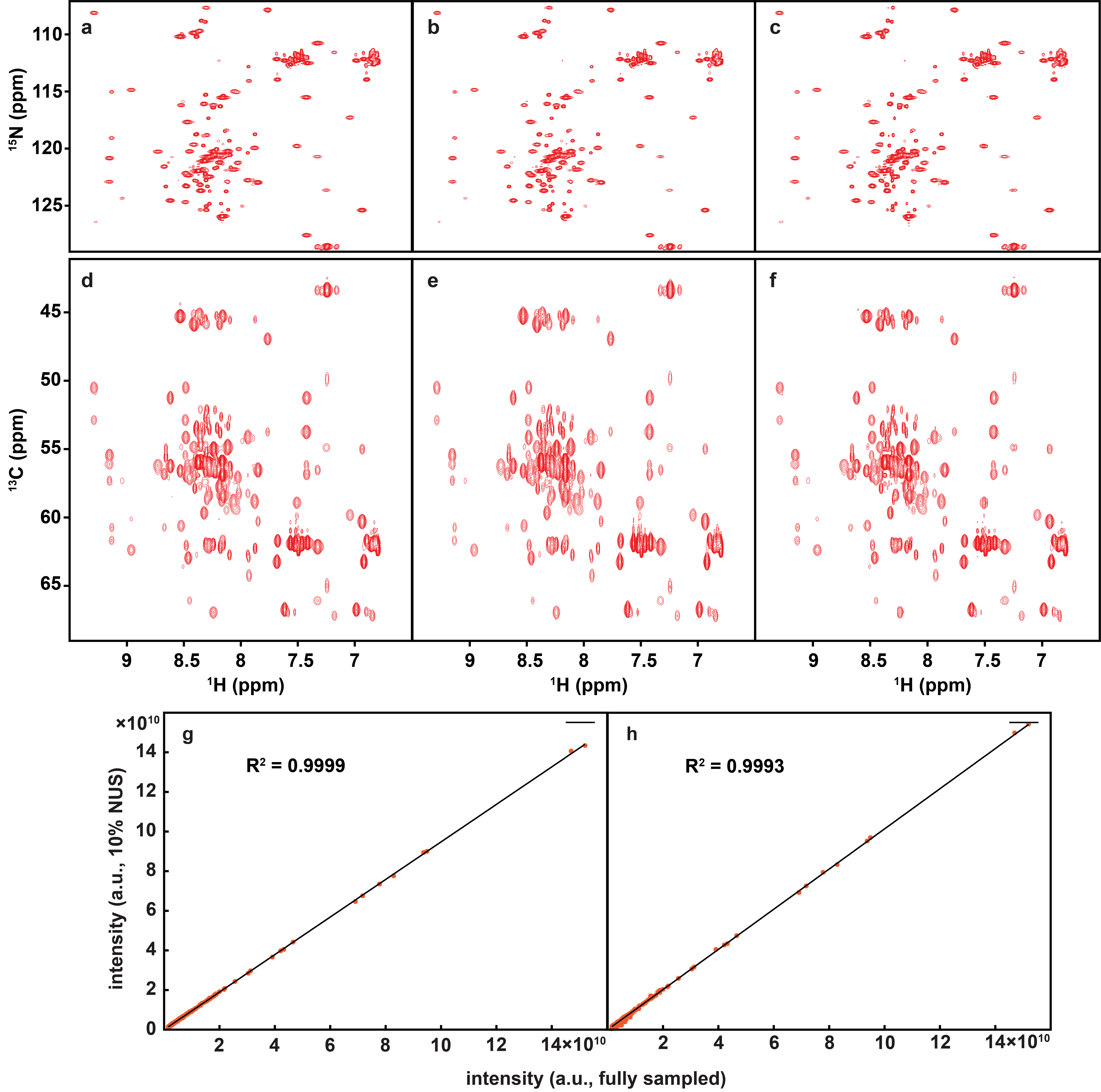
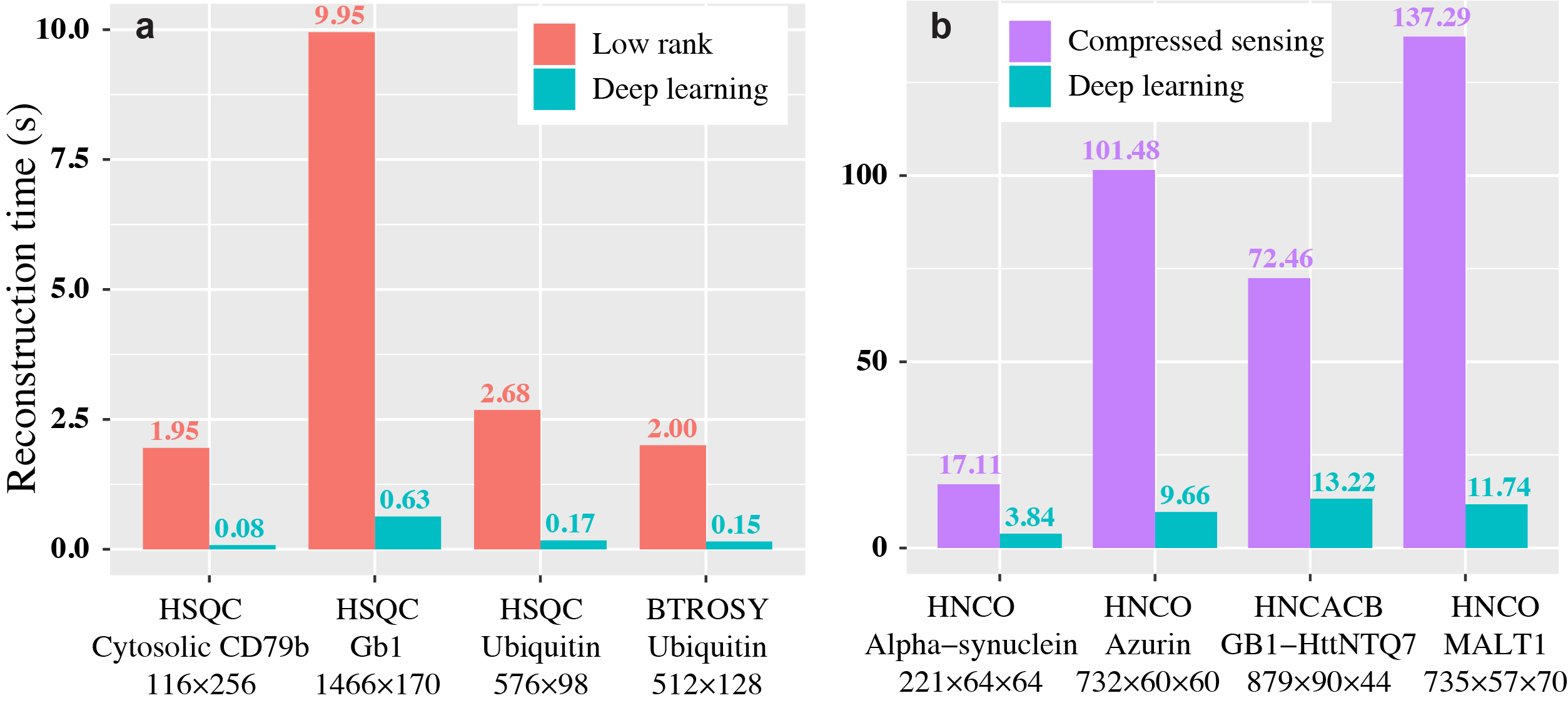
To demonstrate the applicability of trained neural networks, we reconstruct several spectra under NUS, including 2D HSQC spectrum from cytosolic CD79b, 2D HSQC spectrum from ubiquitin, 2D HSQC spectrum from GB1, 2D TROSY spectrum from ubiquitin, 3D HNCO spectrum of azurin protein and 3D HNCACB of GB1-HttNTQ7 protein. The proposed DL NMR will be compared with two state-of-the-art NMR spectroscopy reconstruction approaches, including low rank (LR)² for 2D spectra and compressed sensing (CS)^8-10 for 3D spectra. Pearson correlation coefficient R² is calculated as a measure of the peak intensities difference between the reconstructed spectrum and fully sampled spectrum.
The reconstructed 2D HSQC spectrum from ubiquitin in Fig.2, Pearson correlation coefficient of four 2D spectra in Fig.3 show that: (a) DL achieves the same level of reconstructed 2D ¹H-¹⁵N HSQC spectra quality as LR method does from 25% NUS data and representative peak shapes are closing to the fully sampled peak shapes. (b) At low NUS densities, DL even surpass LR in terms of higher intensity correlations. For two reconstructed 3D spectra in Fig.4 and Fig.5, both DL and CS approaches produce nice reconstructions that are very closing to the fully sampled ones. The peak intensity correlations of DL and CS, with R² > 0.99, shows the high fidelity of reconstruction. Computational time for the reconstructions of 2D spectra and 3D spectra in Fig.6 shows that without compromising the spectra quality, DL is much faster than other state-of-the-art methods such as low rank and compressed sensing. Although the training time is long, which is 5.08 hours for 2D NMR and 31.68 hours for 3D NMR, a unique network can be trained in advance and then applied to reconstruct many spectra that have the same dimensionality (2D or 3D) and do not deviate much in sizes of the spectral dimensions and NUS levels.

Conclusion

In summary, we present the proof-of-concept demonstration of application the deep learning (DL) for fast reconstructing high-quality NMR proteins spectra from NUS data. This result opens an avenue for the application of DL and possibly other artificial intelligence techniques in biological NMR. The training data and deep learning neural network will be shared at Computational Sensing Group at Xiamen University with website address http://csrc.xmu.edu.cn

Acknowledgements

This work was supported in part by the National Natural Science Foundation of China (NSFC) under grants 61571380, 61971361, 61871341 and U1632274, the Joint NSFC-Swedish Foundation for International Cooperation in Research and Higher Education (STINT) under grant 61811530021, the National Key R&D Program of China under grant 2017YFC0108703, the Natural Science Foundation of Fujian Province of China under grant 2018J06018, the Fundamental Research Funds for the Central Universities under grant 20720180056, the Science and Technology Program of Xiamen under grant 3502Z20183053, the China Scholarship Council, the Swedish Research Council under grant 2015–04614 and the Swedish Foundation for Strategic Research under grant ITM17-0218.

The correspondence should be sent to Dr. Xiaobo Qu (Email: quxiaobo@xmu.edu.cn)

References

[1] J. C. Hoch and A. Stern, NMR Data Processing. Wiley, 1996.

[2] X. Qu, M. Mayzel, J. Cai, Z. Chen, and V. Orekhov, "Accelerated NMR spectroscopy with low-rank reconstruction," Angewandte Chemie International Edition, vol. 54, no. 3, pp. 852-854, 2015.

[3] H. M. Nguyen, X. Peng, M. N. Do, and Z. Liang, "Denoising MR spectroscopic imaging data with low-rank approximations," IEEE Transactions on Biomedical Engineering, vol. 60, no. 1, pp. 78-89, 2013.

[4] J. Ying et al., "Hankel matrix nuclear norm regularized tensor completion for N-dimensional exponential signals," IEEE Transactions on Signal Processing, vol. 65, no. 14, pp. 3702-3717, 2017.

[5] J. Ying, J. Cai, D. Guo, G. Tang, Z. Chen, and X. Qu, "Vandermonde factorization of Hankel matrix for complex exponential signal recovery—application in fast NMR spectroscopy," IEEE Transactions on Signal Processing, vol. 66, no. 21, pp. 5520-5533, 2018.

[6] H. Lu et al., "Low rank enhanced matrix recovery of hybrid time and frequency data in fast magnetic resonance spectroscopy," IEEE Transactions on Biomedical Engineering, vol. 65, no. 4, pp. 809-820, 2018.

[7] G. Huang, Z. Liu, L. v. d. Maaten, and K. Q. Weinberger, "Densely connected convolutional networks," in Proceedings of the IEEE Conference on Computer Vision and Pattern Recognition, 2016, pp. 4700-4708.

[8] X. Qu, X. Cao, D. Guo, and Z. Chen, "Compressed sensing for sparse magnetic resonance spectroscopy," in International Society for Magnetic Resonance in Medicine 18th Scientific Meeting, 2010, p. 3371.

[9] K. Kazimierczuk and V. Y. Orekhov, "Accelerated NMR spectroscopy by using compressed sensing," Angewandte Chemie International Edition, vol. 50, no. 24, pp. 5556-5559, 2011.

[10] X. Qu, D. Guo, X. Cao, S. Cai, and Z. Chen, "Reconstruction of self-sparse 2D NMR spectra from undersampled data in the indirect dimension," Sensors, vol. 11, no. 9, pp. 8888-8909, 2011.

Figures

Figure 1.Flowchart of deep learning (DL) NMR spectroscopy.

Figure 2.Reconstruction of a 2D ¹H–¹⁵N HSQC spectrum of cytosolic CD79b protein from the B-cell receptor. (a)-(c) are the fully sampled spectra, LR and DL reconstructions from 25% NUS data, respectively; (d) and (e) are peak intensity correlations obtained by LR and DL methods, respectively; (d) and (e) are zoomed out 1D ¹⁵N traces, and the red, yellow and green lines represent the spectra obtained with fully-sampling, LR and DL methods, respectively. Note: 25% NUS data were used in the reconstruction.

Figure 3.Correlation coefficients for the (a) 2D HSQC spectrum from cytosolic CD79b, (b)2D HSQC spectrum from ubiquitin, (c)2D HSQC spectrum from GB1, (d)2D TROSY spectrum from ubiquitin at different rates of NUS. Note: The green and yellow lines indicate the Pearson correlation coefficient R² of DL and LR methods, each compared with the fully sampled spectrum, respectively. The error bars are the standard deviations of the correlations over 100 NUS resampling trials.

Figure 4.The projections on ¹H-¹⁵N and ¹H-¹³C planes of the 3D HNCO spectra of azurin protein. (a) and (d) are projection spectra of the fully sampled referenced spectrum. (b) and (e) are projection spectra of the CS reconstructed spectrum. (c) and (f) are projection spectra of the DL reconstructed spectrum. (g) and (h) are the peak intensity correlations achieved by CS and DL, respectively. Note: 5% NUS data were acquired for reconstruction. The contours of all projection spectra are at the same level.

Figure 5.The projections on ¹H-¹⁵N and ¹H-¹³C planes of the 3D HNCACB of GB1-HttNTQ7 protein. (a) and (d) are projection spectra of the fully sampled referenced spectrum. (b) and (e) are projection spectra of the CS reconstructed spectrum. (c) and (f) are projection spectra of the DL reconstructed spectrum. (g) and (h) are the peak intensity correlations achieved by CS and DL, respectively. Note: 5% NUS data were acquired for reconstruction. The contours of all projection spectra are at the same level.

Figure 6. Computational time for the reconstructions of (a) 2D spectra and (b) 3D spectra. The spectra type, its corresponding protein and spectra size after routine processing of the direct dimension are listed below each bar.

Proc. Intl. Soc. Mag. Reson. Med. 28 (2020)

3040