Introduction

Carbon atoms are fundamental to metabolism, so tracking carbon nuclei via magnetic resonance has the potential to monitor this key process. Unfortunately, there is too little Carbon present in the human body for conventional Magnetic Resonance Imaging (MRI) techniques. Hyperpolarization increases the signal intensity by approximately 10,000 times [1]. As the carbon atoms move between compounds via metabolism, the relative amounts of each metabolite are observed based on their chemical shift. If done fast enough, we observe metabolite kinetics (e.g. cellular transport, enzyme kinetics). The byproducts can be localized in space-time with imaging. This technique is non-toxic, has no ionizing radiation, and can be performed in volunteers as well as patients [2].

Unlike conventional MR, where the signal recovers after excitation, there is a finite signal energy to exploit when imaging hyperpolarized compounds. This limits the resolution attainable (e.g. images of $$$16\times 16$$$ with $$$4-5$$$ mm per pixel). For presentation, the imagery is interpolated to an observable numbers of pixels; the methods used are most commonly nearest-neighbor or linear interpolation [3]. In a clinical scan, along with imagery of the hyperpolarized compounds, conventional MR proton images are also made. The proton imagery is has much higher resolution than the metabolic imagery. In this work, we use the high-resolution proton imagery to inform the interpolation of the metabolic imagery.

Methods

Prior to transferring information from the proton imagery to the metabolic imagery, we must first accommodate differences in the dynamic ranges of the images. Both images are scaled so that their values lie in the $$$[0,1]$$$ interval: $$$I_H=\hat{I}_H/\max(\hat{I}_H)$$$ and $$$I_L=\hat{I}_L/\max(\hat{I}_L)$$$, where $$$\hat{I}_H\in\mathbb{R}^{M_H\times N_H}$$$ and $$$\hat{I}_L\in\mathbb{R}^{M_L\times N_L}$$$ are the original high and low resolution images, respectively. Once scaled, we will make the gradient of the interpolated metabolic image similar to the gradient of thehigh-resolution proton image: $$$\nabla I_M \approx \nabla I_H$$$.The interpolated imagery is the result of the following optimization problem with two terms in its objective function.

\begin{equation}\begin{aligned}
\underset{I_M}{\text{minimize}} &\hspace{8pt} \frac{1}{2} \| D\left(B I_M\right) - I_L \|_2^2 + \frac{\lambda}{2}\left\| \nabla I_M - \nabla I_H \right\|_{w,2}^2 \\
\text{subject to} &\hspace{8pt} I_M \geq 0
\end{aligned}\end{equation}

The first term is a data consistency term that minimizes the difference between $$$D(B\,I_M)$$$ and $$$I_L$$$ where $$$I_M$$$ is the interpolated metabolic image, $$$I_L$$$ is the reconstructed low resolution image, $$$B$$$ is the blurring operator (note that since we know the trajectory used to collect the data, the blurring operator is known), and $$$D$$$ is a downsampling operator. The second term minimizes the weighted norm of the difference of the gradients of $$$I_M$$$ and the high-resolution proton image $$$I_H$$$. The regularization parameter $$$\lambda$$$ is chosen by the user to choose the relative effects of the terms in the objective function. The images are of the magnitudes of the received signal; therefore, the $$$I_M\geq 0$$$ non-negativity constraint is imposed as well. The vector $$$w$$$ is the the result of linearly interpolating the low-resolution metabolic image $$$I_L$$$ to the size of the high-resolution $$$I_M$$$. These weights are used so that the gradients do not cause artifacts in areas of the image where there is significant proton signal but without much of the hyperpolarized compound.

The problem presented is a convex optimization problem; a solution can be determined with known algorithms and existing software solutions. The form of this problem is appropriate for the Fast Iterative Shrinkage Threshold Algorithm (FISTA). A beneficial property of this algorithm is that it exhibits quadratic convergence, requiring fewer iterations than first order methods. We choose to solve it using FISTA with line search for convergence in fewer iterations.

Results

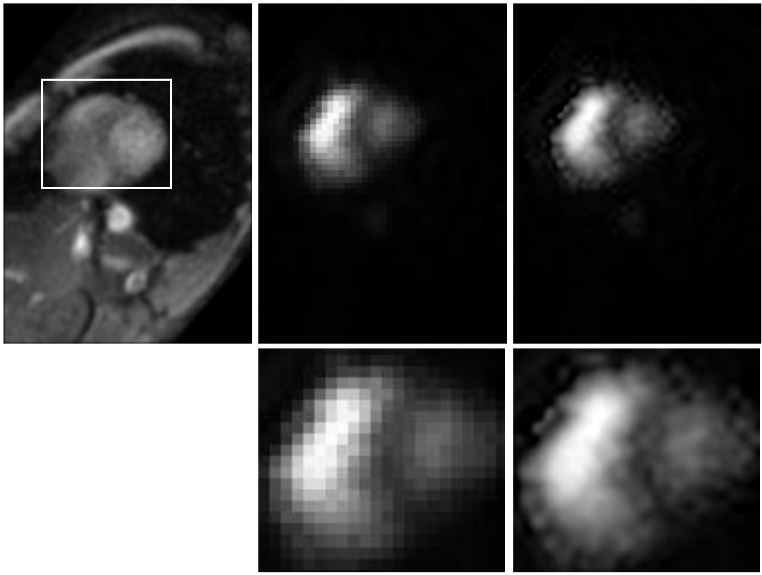
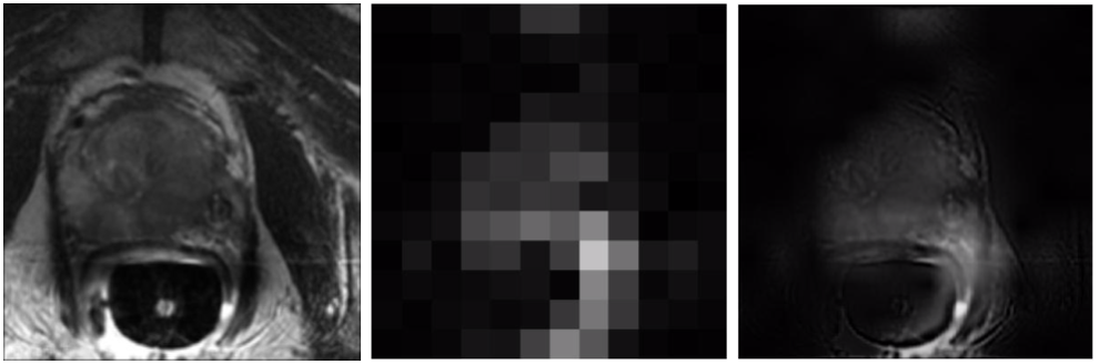
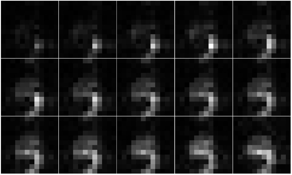
Figure 1 shows a slice of the cardiac study: a T2 weighted image, an image of the hyperpolarized pyruvate, and the interpolated image of the hyperpolarized pyruvate. The region enclosed in the white box on the T2 weighted image is displayed in the second row of the figure.Note the additional detail presented in the interpolated image.

Figure 2 shows imagery of the hyperpolarized pyruvate for the prostate slice of Fig. 1. Images are separated by $$$2$$$ seconds; they are ordered from left-to-right and top-to-bottom).

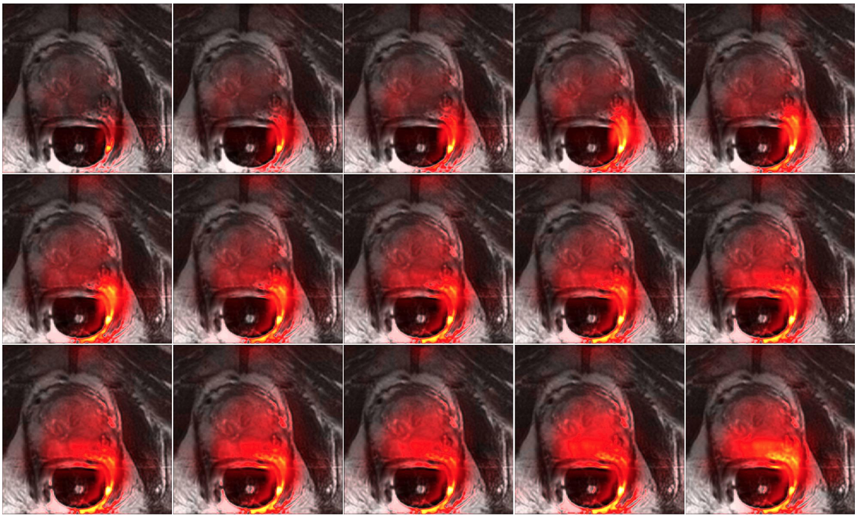
In fig. 3, the di-chromatic interpolated imagery is converted to a false color image and then fused with the original T2 weighted proton imagery using the CLS fusion algorithm [4]. (This fusion algorithm retains color while incorporating spatial information during fusion; this is especially important for false color imagery, like that used here, where the color corresponds to a quantitative value.)

Conclusion

In this work, we present the di-chromatic interpolation algorithm that informs the interpolation of a low-resolution metabolic image with the details of a high-resolution proton image. The interpolated image permits a better understanding of the location of the metabolic activity.

Acknowledgements

No acknowledgement found.