Introduction

Unlike MRI neuroimaging, MR spectroscopy lacks standard analysis pipelines, which substantially hinders use in research. For fitting of post-processed data, a number of expert-created programs are available (1-3), but many suffer from a closed-source approach, or require high levels of user interaction, or have significant expense. The currently available software is not easily extensible to new uses of MRS such as high voxel count MRSI or time-series modelling of fMRS.

Here we introduce a new Python-based MRS fitting tool, FSL-MRS, working on the principle of linear combination of pre-calculated basis spectra. This tool calculates full posterior distributions of the fitted metabolite concentrations to estimate concentration covariances and uncertainties. FSL-MRS incorporates an interactive reporting interface which uses the latest data-science visualisation tools. The tool is open source, free as part of the FSL software package, and operates with a command line or configuration-file interface.

In this work we show an initial implementation of the user interface and output and describe the fitting model and approach. A validation of the tool’s concentration estimates is carried out in a uniform phantom, and its in vivo performance is assessed in three brain regions of 37 subjects at 7T.

Methods

The model for the complex-domain spectrum is $$Y(\nu)=B(\nu)+exp[i(\phi_0+\nu\phi_1)]\sum_{g=1}^{N_G}\sum_{l=1}^{N_g}C_{l,g}M_{l,g}(\nu;\gamma_g,\epsilon_g)$$
$$M_{l,g}(\nu;\gamma_g,\epsilon_g) = \mathcal{F}\left \{ m_{l,g}(t)exp[-(\gamma_g+i\epsilon_g)t]) \right \}$$
where $$$B(\nu)$$$ describes an n^th-order polynomial estimate of the baseline, the second term applies a global phase term and the final term is the sum of all scaled, shifted and broadened metabolite basis spectra $$$M_{l,g}(\nu;\gamma_g,\epsilon_g)$$$. To avoid overfitting there is no flexibility in the metabolite line-shapes beyond shifting (ε) and broadening (γ), which can be flexibly applied to N_G groups of metabolites (all metabolites in a group are treated with the same ε and γ). $$$\mathcal{F}$$$ is the Fourier transform and $$$m_{l,g}(t)$$$ is the inverse Fourier transform of $$$M_{l,g}(\nu;0,0)$$$ and equivalent to the raw time-domain basis functions generated.

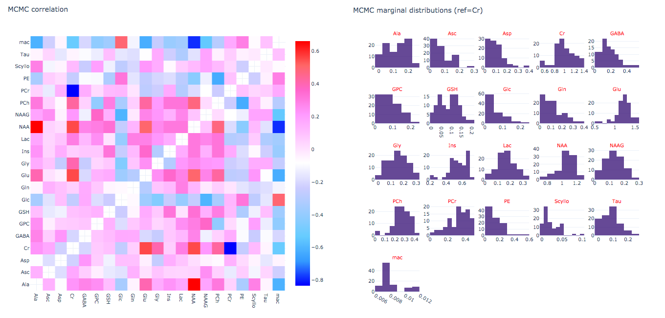
Initialization is achieved using the truncated Newton algorithm in the SciPy package. The final fit is carried out over all model parameters using Metropolis-Hastings (a Markov chain Monte Carlo algorithm). An interactive HTML report (Plotly, Montreal, Canada) is generated for each fit displaying the fitted spectrum, model fit, residuals and concentrations (Fig 1) and concentration posterior distributions, metabolite covariances and scaled basis spectra (Fig 2).

Validation of water scaled concentrations was carried out in a uniform aqueous phantom (SPECTRE, Gold Standard Phantoms, London, UK) containing six metabolites (NAA, Cr, Cho, Ins, Glu and Lac) using a previously published STEAM sequence at 7T (4,5). The same basis spectra were used to estimate the concentrations of six metabolites from 5 Hz line-broadened spectra from the phantom. Absolute concentrations were calculated from referencing the integral of the scaled creatine spectrum to an un-suppressed water spectrum taken to be equivalent to 55 M concentration.

In vivo performance was compared to LCModel (2) in three brain regions (ACC, OCC and putamen) in 37 subjects scanned using a STEAM sequence protocol in a whole body 7T scanner (Siemens, Erlangen, Germany). Fitting basis sets were created by density matrix simulation of 20 metabolites using an extended 1D-projection method (6) in Spinach (7) with an in vivo measured macromolecular basis spectrum. LCModel was used without concentration ratio priors.

Results

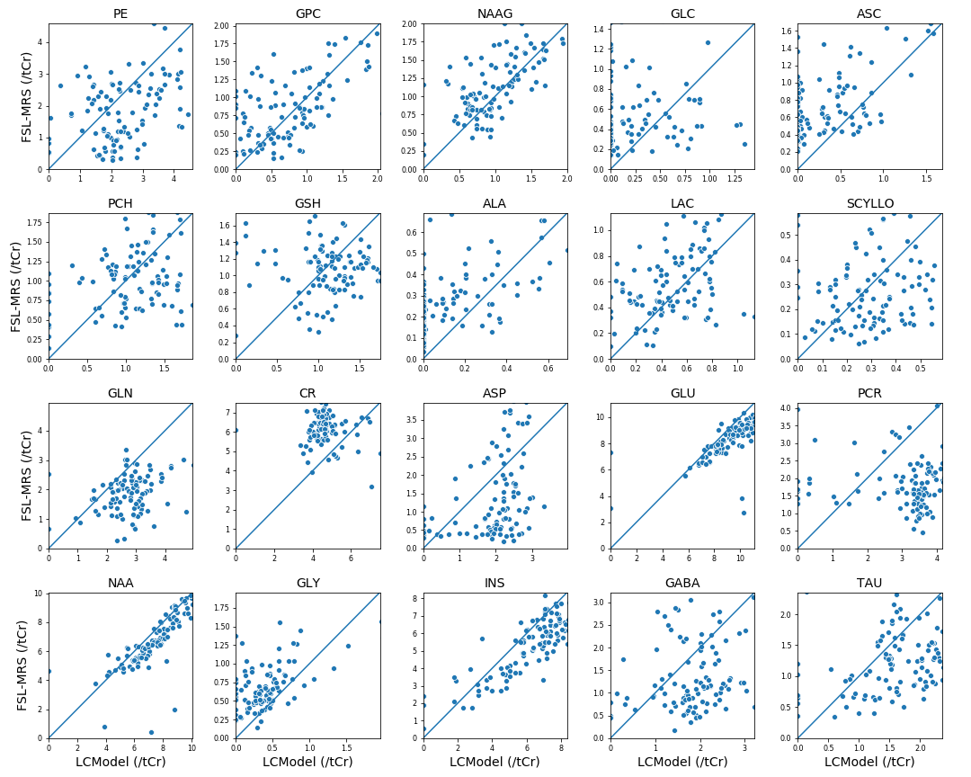
Results of the validation of concentration estimates are displayed in Figure 3. FSL-MRS correctly estimates the water-scaled metabolite concentrations of three of six included metabolites. This appears to match the performance of LCModel (ignoring a global scaling offset seen with LCModel in this case).

The per-metabolite correlation plots between FSL-MRS and LCModel are shown in Figure 4. Concentrations are expressed relative to total creatine and scaled so that total creatine equals 8. The mean Pearson correlation is 0.27. In the most prominent metabolites (NAA, Ins, PCh and Glu) correlation was 0.59.

Discussion

Here we presented an initial implementation of FSL-MRS, demonstrating equivalence to a single existing tool. Work will continue to evaluate with simulation data to confirm validity and against other toolboxes in a wider set of data (different field strengths and sequences and pathological subjects).

We will take advantage of the tool’s flexibility to handle MRSI and incorporate time series modelling to fit fMRS. This will also incorporate reading data from multiple formats, including ascii and 4D NIfTI. We will also extend the current line-shape model to incorporate a distribution of Lorentzian resonances.

We plan to distribute FSL-MRS in 2020.

Acknowledgements

We thank Phil Cowen and Beata Godlewska for providing the test data, which was funded by the MRC [MR/K022202/1]. The Wellcome Centre for Integrative Neuroimaging is supported by core funding from the Wellcome Trust (203139/Z/16/Z).