2854
Separation of Metabolite and Macromolecule Signals for Short-TE $$$^1$$$H-MRSI Using Learned Nonlinear Models1Department of Bioengineering, University of Illinois at Urbana-Champaign, URBANA, IL, United States, 2Beckman Institute for Advanced Science and Technology, University of Illinois at Urbana-Champaign, URBANA, IL, United States
Synopsis
We report a novel method to separate metabolite and macromolecule signals from short-TE $$$^1$$$H-MRSI data using learned nonlinear low-dimensional models. A deep-learning-based strategy was developed to learn the nonlinear low-dimensional manifolds where the metabolite and MM signals reside, respectively. A constrained reconstruction formulation is proposed to incorporate the learned model as a prior to reconstruct and separate metabolite and MM signals. The performance of the proposed method was evaluated using both simulation and experimental short TE $$$^1$$$H-MRSI data. Promising results have been obtained, demonstrating the potential of the proposed method in addressing this challenging problem.
Introduction
Short-TE MRSI offers improved SNR, detection, and quantification of short-T$$$_2$$$ and J-coupled molecules$$$^{1,2}$$$. However, the presence of macromolecule (MM) signals at short TEs (spectrally overlaps with metabolite signals) is a major challenge for data processing. Inaccurate separation of the metabolite and MM signals can adversely affect the quantitative analysis of MRSI data$$$^{3}$$$. The typical approach to address the separation problem is to use a parametric model and fit the two components by estimating the respective model parameters$$$^{4-6}$$$. However, this approach offers limited performance and is sensitive to noise and model errors. We present here a novel method to separate metabolite and MM signals in short-TE MRSI data by integrating physics-based modeling and machine learning. Specifically, we proposed a deep autoencoder (DAE)$$$^{7}$$$ to learn metabolite and MM-specific nonlinear low-dimensional models by exploiting their unique spectral features. A regularized reconstruction formulation was proposed to incorporate the learned models to reconstruct and separate the two signal components. The effectiveness of the proposed method has been evaluated using simulated and experimental data. Promising results were obtained.Theory and Methods: Problem Formulation
The spatiotemporal function in short-TE $$$^1$$$H-MRSI can be expressed as:$$\rho(\mathbf{r},t) = \rho_{met}(\mathbf{r},t)+\rho_{mm}(\mathbf{r},t)\quad\quad\quad\quad\quad\quad\quad[1]$$where $$$\rho_{met}(\mathbf{r},t)$$$ and $$$\rho_{mm}(\mathbf{r},t)$$$ denote the metabolite and MM signals, respectively. The goal is to estimate $$$\rho_{met}$$$ and $$$\rho_{mm}$$$ from $$$\rho$$$, which is an ill-posed problem. However, it has been well established that the signal at each voxel can be parametrically modeled as:$$s(t)= \sum_{m=1}^{M}c_me(t,\boldsymbol{\theta}_m)\phi_m(t)h(t) +\sum_{l=1}^Lb_lM_l(t,\boldsymbol{\beta}_l).\quad\quad\quad\quad\quad[2]$$The first term captures the metabolites and $$$c_m$$$, $$$e(t,\boldsymbol{\theta}_m)$$$, $$$\phi_m(t)$$$, and $$$h(t)$$$ are the $$$m$$$-th molecule's concentration, spectral variation parameterized by $$$\boldsymbol{\theta}_m$$$ (e.g., $$$T_2^*$$$ and $$$\delta f$$$), resonance structure, and lineshape distortion. The second term represents the MMs where $$$b_l$$$ and $$$M_l(t,\boldsymbol{\beta}_l)$$$ denote the intensity and lineshape (Gaussian) for the $$$l$$$-th MM group (linewidths $$$\boldsymbol{\beta}_l$$$). Conventionally, separation is done by quantifying $$$c_m$$$, $$$\boldsymbol{\theta}_m$$$, $$$b_l$$$, and $$$\boldsymbol{\beta}_l$$$ from $$$s(t)$$$ and constructing each component using the estimated parameters$$$^{4-6}$$$.Recognizing the distinct spectral characteristics of $$$\rho_{met}(\mathbf{r},t)$$$ and $$$\rho_{mm}(\mathbf{r},t)$$$, we propose to use DAEs to model each signal. These learned DAEs are expected to capture metabolite and MM-specific low-dimensional manifolds which can be used as priors for their separation. This is different from other deep-learning-based strategies that learn an end-to-end mapping from noisy short-TE data to separated metabolite and MM signals directly$$$^{8,9}$$$. In these strategies, the networks need to capture the underlying spectral features as well as all the variations due to noise, artifacts, and acquisition parameters. Specifically, denoting $$$\mathcal{N}_{met}$$$ and $$$\mathcal{N}_{mm}$$$ as the DAEs trained to capture the metabolite and MM-specific manifolds and $$$\mathbf{X}=\mathbf{X}_{met}+\mathbf{X}_{mm}$$$ the matrix representations of the spatiotemporal functions, we formulate the signal separation problem as:$$ \{\hat{\mathbf{X}}_{met},\hat{\mathbf{X}}_{mm}\}=\arg\min_{\mathbf{X}_{met},\mathbf{X}_{mm}}\|\mathbf{d}-\Omega\{\mathbf{FB}\odot\mathbf{X}\}\|_2^2 + \lambda_1\sum_{n=1}^N\|\mathcal{N}_{met}(\mathbf{X}_{met}^n)-\mathbf{X}_{met}^n\|_2^2+ \lambda_2\sum_{n=1}^N\|\mathcal{N}_{mm}(\mathbf{X}_{mm}^n)-\mathbf{X}_{mm}^n\|_2^2+ \lambda_3R(\mathbf{X})\quad[3]$$where $$$\mathbf{F}$$$ represents Fourier transform, $$$\mathbf{B}$$$ models the $$$B_0$$$ inhomogeneity, $$$\Omega$$$ a sampling operator, and $$$\mathbf{d}$$$ the acquired $$$(k,t)$$$-space data (water/lipids removed). The first two regularization terms enforce the constraints that metabolites and MMs follow the low-dimensional representations captured by $$$\mathcal{N}_{met}$$$ and $$$\mathcal{N}_{mm}$$$. The last term is a spatial constraint (e.g., weighted-$$$\ell_2$$$ or $$$\ell_1$$$ penalty$$$^{10}$$$). An efficient ADMM (alternating direction method of multiplier) algorithm was developed to solve this problem $$$^{11}$$$ (details omitted due to space limitation).
Theory and Methods: Network Training and Design
We used the DAE architecture described in (11). A special strategy is devised to train $$$\mathcal{N}_{met}$$$ and $$$\mathcal{N}_{mm}$$$. Specifically, the training is done by:$$\{\hat{\boldsymbol{\theta}}_{met}\} = \arg\min_{\boldsymbol{\theta}_{met}}\frac{1}{N} \sum_{n=1}^N\left[\epsilon(\mathbf{x}_{met}^n-\mathcal{N}_{met}(\mathbf{x}_{met}^n;\boldsymbol{\theta}_{met}))+\|\mathcal{N}_{met}(\mathbf{x}_{mm}^n;\boldsymbol{\theta}_{met})\|_2^2 \right]\quad\quad\quad\quad\quad[4]$$where $$$\{\mathbf{x}^n_{met}\}$$$ and $$$\{\mathbf{x}^n_{mm}\}$$$ are the metabolite and MM training data, $$$\boldsymbol{\theta}_{met}$$$ contains the parameters for the metabolite-specific network, and $$$\epsilon$$$ a loss function (e.g., mean-square-error). The regularization term penalizes the representation of the metabolite network for MM signals. Same idea is applied for the MM network. This enforces the DAE to learn a representation specific to one signal component with minimal representation power of the other. Training data was generated using Eq.[1] with $$$\phi_m(t)$$$ from quantum-mechanical simulations and $$$c_m$$$, $$$\boldsymbol{\theta}_m$$$, $$$b_l$$$, and $$$\boldsymbol{\beta}_l$$$ randomly sampled from distributions constructed using literature and experimental values$$$^{8,12,13}$$$.Results
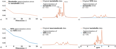
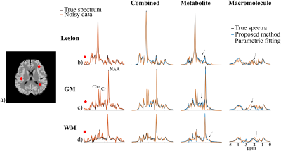
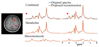
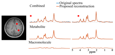
Figure 1 demonstrates the accurate component-specific approximations achieved by the trained DAE using simulated $$$^1$$$H-MRSI data (both overall relative $$$\ell_2$$$ errors and representative spectra). The metabolite network is shown to capture the metabolite component accurately, but the MM component poorly, vice versa for the MM network. A set of metabolite and MM separation results from a numerical phantom are shown in Fig. 2. The phantom contains spatially varying metabolite and MM spectra with different concentrations, lineshapes, frequency shifts, and a lesion-like feature. Results from a parametric fitting method (QUEST) was also obtained$$$^{6}$$$. We can clearly observe that although the proposed method and parametric fitting produced similar overall spectra (metabolite + MM), the proposed method offers significantly improved accuracy for the separated metabolite and MM components (Fig. 2b-d). Figure 3 shows the results from a set of in vivo short-TE FID-CSI data from a healthy volunteer (3T scanner). As can be seen, the proposed method successfully separated the metabolite and MM spectra from the original data. We also applied the proposed method to the truncated FID and produced a negligible MM component (Fig. 4), indicating the robustness of the proposed method.Summary
A new learning-based method that exploits the nonlinear low-dimensional models of metabolites and MMs was proposed for their separation in short-TE $$$^1$$$H-MRSI. Simulation and experimental results demonstrated the effectiveness of the proposed method.Acknowledgements
No acknowledgement found.References
1. Bogner W, Gruber S, Trattnig S, et al. High-resolution mapping of human brain metabolites by free induction decay 1H MRSI at 7 T. NMR Biomed, 25(6):873–882, 2012.
2. Scheenen TWJ, Klomp DWJ, Wijnen JP, et al. Short echo time 1H-MRSI of the human brain at 3T with minimal chemical shift displacement errors using adiabatic refocusing pulses. Magn Reson Med, 59(1):1–6, 2008.
3. Birch R, Peet AC, Dehghani H, et al. Influence of macromolecule baseline on 1H MR spectroscopic imaging reproducibility. Magn Reson Med, 77(1):34–43, 2017.
4. Cudalbu C, Mlynarik V, and Gruetter R. Handling macromolecule signals in the quantification of the neurochemical profile. J Alzheimer Dis, 31(s3):S101–S115, 2012.
5. Provencher SW. Automatic quantitation of localized in vivo 1H spectra with LCModel. NMR Biomed, 14(4):260–264, 2001.
6. Ratiney H, Coenradie Y, Cavassila S, et al. Time-domain quantitation of 1H short echo-time signals: background accommodation. Magn Reson Mater Phys Biol Med, 16(6):284–296, 2004.
7. Hinton GE and Salakhutdinov RR. Reducing the dimensionality of data with neural networks. Science, 313(5786):504–507, 2006.
8. Lee HH and Kim H. Intact metabolite spectrum mining by deep learning in proton magnetic resonance spectroscopy of the brain. Magn Reson Med, 82(1):33–48, 2019.
9. Gurbani SS, Sheriff S, Maudsley AA, et al. Incorporation of a spectral model in a convolutional neural network for accelerated spectral fitting. Magn Reson Med, 81(5):3346–3357, 2019.
10. Lam F, Ma C, Clifford B, et al. High-resolution 1H-MRSI of the brain using SPICE: data acquisition and image reconstruction. Magn Reson Med, 76(4):1059–1070, 2016.
11. Lam F, Li Y, and Peng X. Constrained magnetic resonance spectroscopic imaging by learning nonlinear low-dimensional models. IEEE Trans Med Imaging, 2019.
12. Lam F, Li Y, Guo R, et al. Ultrafast magnetic resonance spectroscopic imaging using SPICE with learned subspaces. Magn Reson Med, 2019.
13. Li Y, Lam F, Clifford B, et al. A subspace approach to spectral quantification for MR spectroscopic imaging. IEEE Trans Biomed Eng, 64(10):2486–2489, 2017.
Figures


