Purpose

This work aims to recover high quality MRS from its noise-corrupted FID signals. This corruption may be caused by magnetic field strength, sample or electronics temperature, etc.[1], which makes re-sampling become a common approach to enhance the Signal-to-Noise Ratio (SNR) of MRS signal. In order to reduce the long acquisition time caused by re-sampling, several denoising methods[2-4] based on Hankel matrix, such as Cazdow’s method[2], have been proposed. However, MRS denoising is suffering from the setting of the prior parameter, which is unknown in applications and difficult to estimate accurately. This work is based on a denoising method that explores the low-rank property of the Hankel matrix transformed from the FID, and provides an accurate estimate on the noise bound to make this approach become a denoising method with auto-setting parameter.

Method

In MRS, FID signals are commonly modeled as a sum of several exponentials with decay[5-8]. Let $$$x_{0}{\in}\mathbb{C}^{2N+1}$$$ be a one-dimensional FID
$$ x_{0}(t_{n})=\sum_{r=1}^{R}a_{r}e^{\left({j2{\pi}f_{r}-{\tau}_{r}}\right)t_{n}}, \ n=1,\ldots,2N+1, (1)$$
where $$$a_r$$$, $$$f_r$$$ and $$${\tau}_r$$$ are the amplitude, central frequency and decay factor of the $$$r^{th}$$$ exponential, respectively.
In applications, the measurement is usually corrupted by noise and one receives$$\mathbf{y}=\mathbf{x}_{0}+\mathbf{z}, (2)$$where $$$\mathbf{z}$$$ denotes a Gaussian noise with mean 0 and variance $$${\sigma}^2$$$.
Recently, Qu. et al [6, 9, 10] proposed a signal reconstruction method based on the low-rank property of Hankel matrix converted by FID. This method is called Convex Hankel IOw Rank matrix approximation for Denoising exponential signals (CHORD), where one solves the following optimization problem
$$\min_{\mathbf{x}} \left\|{\mathcal{R}\mathbf{x}}\right\|_{*}+\frac{\lambda}{2}\left\|{\mathbf{y}-\mathbf{x}}\right\|_{2}^{2}, (3)$$
where $$$\mathcal{R}$$$ denotes an operator that transforms a vector into a square Hankel matrix.This method does not require to estimate the rank of Hankel matrix as a prior parameter, and merely owns one regularization parameter, $$$\lambda$$$, whose choice decides the final denoising effect. Therefore, how to set an appropriate $$$\lambda$$$ has become a critical issue. Here, we determine the optimal solution of Eq. (3) through sub-gradient, a bound of $$$\lambda$$$ is obtained, which makes sure that the noise will be removed well when $$$\lambda$$$ lies below this bound,
$$\lambda\leq\frac{2}{\left\|\mathbf{Z}\right\|_{2}}, (4)$$
where $$$\mathbf{Z}$$$ is a weighted Hankel matrix converted by $$$\mathbf{z}$$$, and defined as
$$\mathbf{Z}=\left[ \begin{array}{cccc} z_1 & \frac{z_2}{2} & \cdots & \frac{z_{N+1}}{N+1} \\ \frac{z_2}{2} & \frac{z_3}{3} & \cdots & \frac{z_{N+2}}{N} \\ \vdots & \vdots & \cdots & \vdots \\ \frac{z_{N+1}}{N+1} & \frac{z_{N+1}}{N+1} & \cdots & z_{2N+1} \end{array} \right].(5)$$
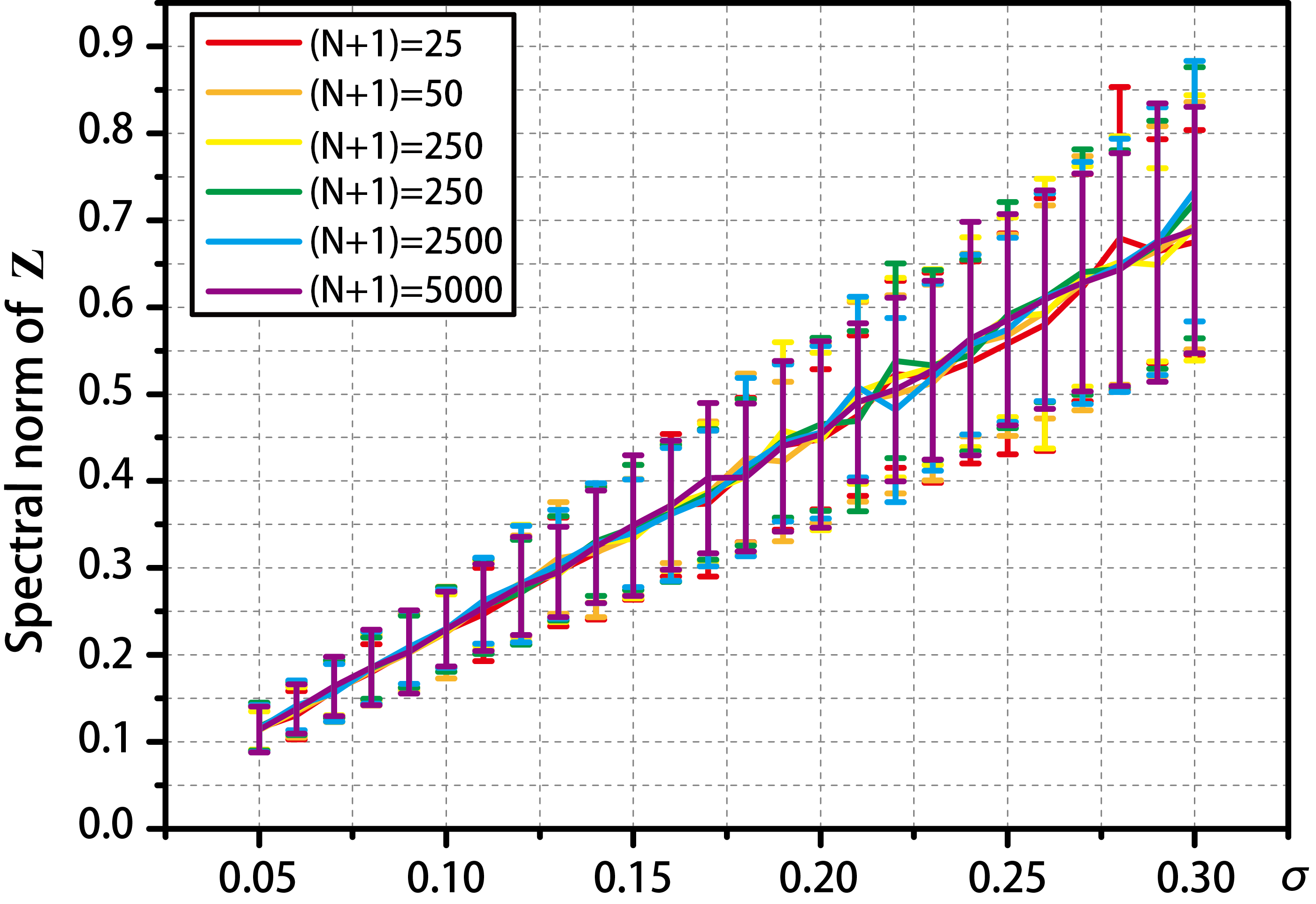
We use a series of $$$\mathbf{z}$$$ with different lengths and variances to explore the relation between the noise and $$$\lambda$$$. The results in Fig. 1 shows that the average of the spectral norm is proportional to the standard deviation of noise. According to Eq. (4), if $$$2/{\lambda}$$$ lies in the region above the lower bound of the $$$\left\|\mathbf{Z}\right\|_{2}$$$, almost all the noise can be removed. Consequently, it is necessary to explore the spectral norm of $$$\mathbf{Z}$$$, especially the lower bound.
We prove that the bound estimate of the expectation of $$$\left\|\mathbf{Z}\right\|_{2}$$$ is as follows
$${\sigma}\sqrt{2C_{\mathbf{w}}\log\left({2N+2}\right)}\geq\mathbb{E}{\left\|{\mathbf{Z}}\right\|_{2}} \geq\frac{C(N+1)\sigma}{2N+1}\sqrt{R_{N}^{2}\left({1+\log\frac{R_{N}^{4}}{Q_{N}^{4}}}\right)}, (6)$$
where $$$C_{\mathbf{w}} = \max(\sum_{n=0}^{N}{w_{n}^{-2}},\sum_{n=1}^{N+1}{w_{n}^{-2}},\ldots,\sum_{n=N}^{2N}{w_{n}^{-2}})$$$, and $$$\mathbf{w}\in\mathbb{R}^{2N+1}$$$ is the weighted in Eq. (5), and defined as $$$\mathbf{w}=\left[{\begin{array}{ccccccc} 1 & 2 & \cdots & N+1 & \cdots & 2 & 1\end{array}}\right]^{T}$$$. $$$R_{N}$$$ and $$$Q_{N}$$$ are two sequences defined as
$$\begin{equation}R_{N}=\sqrt{\sum_{k=0}^{2N}\left|{d_k}\right|^{2}}, \text{and} Q_{N}=\sqrt[4]{\sum_{k=0}^{2N}\left|{d_k}\right|^{4}},(7)\end{equation}$$
where $$$ d_{k}= \left\{ \begin{array}{ll} \frac{2}{(k+1)(k+2)}\sum_{m=0}^{k}\frac{1}{m+1}, 0\leq k\leq N \\[1mm] \frac{2}{(2N-k+1)(k+2)}\sum_{m=k}^{2N}\frac{1}{m-N+1}, N<k\leq 2N \\[1mm] \end{array} \right. $$$.
$$$C$$$ denotes a constant independent of $$$N$$$, and its empirically optimal value lies in 1.2.
In applications, users hope to preserve signal details as much as possible in order to qualify and evaluate the signal. Therefore, we choose to adopt the lower bound we estimate, i.e.,
$$\lambda=\frac{2N+1}{0.6(N+1)\sqrt{R_{N}^{2}\left({1+\log\frac{R_{N}^{4}}{Q_{N}^{4}}}\right)}}\frac{1}{\sigma}.(8)$$

Results

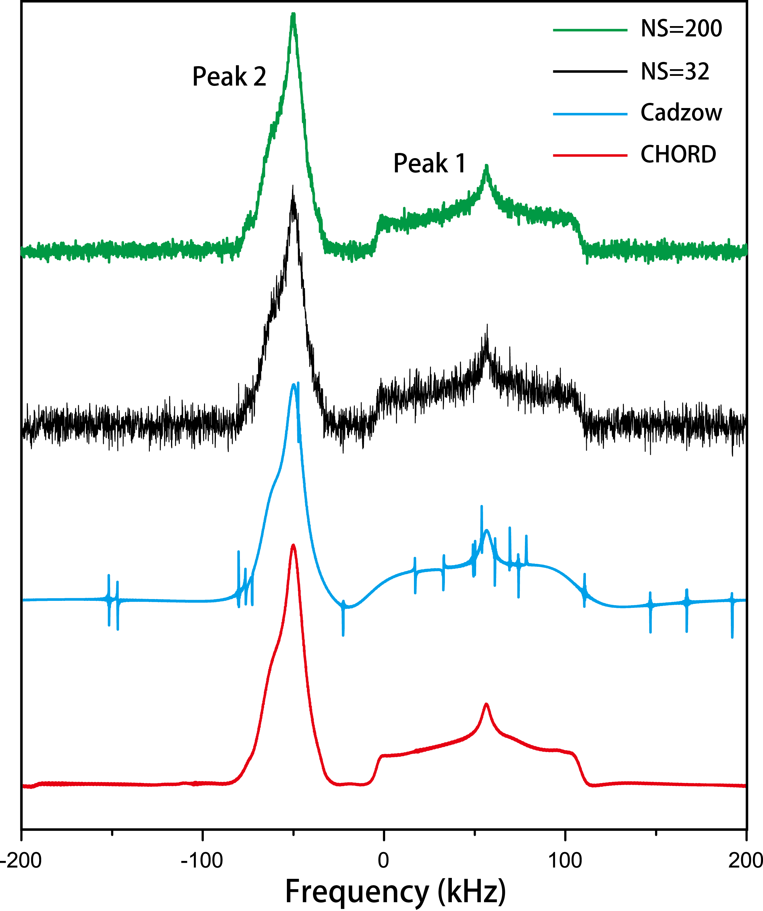
Here we adopt CHORD with auto-setting parameter to denoise a 1D solid-state spectrum from the noise, and compare the denoising results with Cadzow method. Fig. 2 shows denoising results on real solid state data, a static CSA spectrum with the sample of glycine. Compared to Cadzow method, CHORD owns the comparable ability of denoising, keeping high accuracy of line shape. Besides, some fake peaks appear in the denoising results of Cadzow. Consequently, the observations of CSA spectra imply that the CHORD with an appropriate parameter takes merely 16% (NS=32) of the original time to achieve better results of maximally averaged signal (NS=200).

Conclusion

Based on CHORD, a denoising method based on Hankel low-rankness of the complex exponential signals, we attempt to find the bound of the regularization parameter, determine the empirical optimal constant, and estimate the standard derivation of the noise, so that the users are able to apply CHORD with an automatically setting parameter. Experiments on real solid-state MRS data demonstrate that CHORD with the auto-setting parameter achieves more robust and accurate results compared to Cadzow method. It is expected to extend the 1D denoising model into higher dimensional denoising or reconstruction issue.

Acknowledgements

This work was supported in part by National Natural Science Foundation of China (61971361, 61571380, 61871341, 61811530021, U1632274, 61672335), National Key R&D Program of China (2017YFC0108703), Natural Science Foundation of Fujian Province of China (2018J06018), Fundamental Research Funds for the Central Universities (20720180056), Science and Technology Program of Xiamen (3502Z20183053), and China Scholarship Council.The correspondence should be sent to Dr. Xiaobo Qu (Email: quxiaobo@xmu.edu.cn)