INTRODUCTION

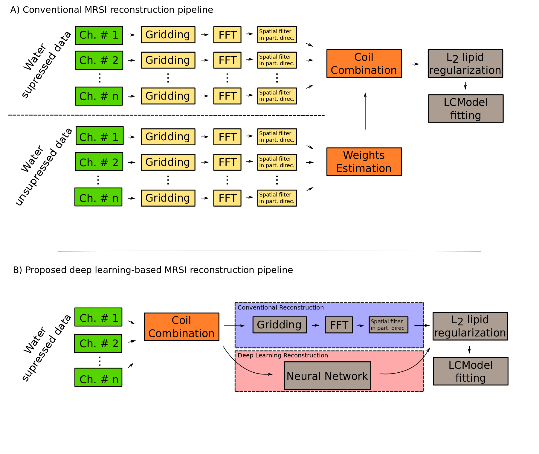
Recently, the combination of spatial-spectral encoding and multi-channel acquisition allowed measuring whole-brain MRSI in clinically attractive scan times¹(~3-15minutes). However, this approach generates large amounts of raw data(up to 100GB for 80x80x47 voxels with 512 spectral points and 32 receive channels), which makes post-processing very time-consuming(e.g., several hours). The conventional post-processing pipeline is depicted in Fig.1.A. To speed up the reconstruction of such data, deep learning could be applied, which is known for computationally extensive training and fast interference. Several deep learning methods for reconstruction of MRI have already been proposed². AUTOMAP³ provides a solution in which the image space domain data are reconstructed from single channel non-Cartesian kSpace data. Such an end-to-end reconstruction approach simplifies the whole reconstruction pipeline but requires the combination of multi-channel data to a single channel in kSpace domain. The purpose of our study was therefore to replace the conventional pipeline from Fig.1.A by the pipeline from Fig.1.B,which would allow a significant speed-up of the reconstruction.

METHODS

AUTOMAP reconstruction

A resolution phantom was measured at a 7T whole-body MR scanner (Magnetom, Siemens, Erlangen, Germany) with a single channel volume coil. A Concentric Ring Trajectory-based FID-MRSI sequence⁴ was used: FOV=220x220mm², matrix=80x80, vector size=72, spectral bandwidth=699Hz, TA=30s.
AUTOMAP was trained on T1-weighted images with synthetic phase derived from the Human Connectome Project⁵. Each of N=40000 images was normalized to a random constant c_n , with 0.6 <|c_n|<1.2, to mimic oscillation of FID signals and non-Cartesian kSpace values were calculated by DFT.
The AUTOMAP’s proposed architecture was used with the change of the activation functions to tanh account for negative values in real and the imaginary part. Two networks were trained to reconstruct the real/imaginary part of the signal with parameters: Learning_rate=0.00002, Number_of_epochs=100, optimizer=RMSprop, momentum=0, decay=0. This approach was compared with the conventional reconstruction based on iterative Pipe-Menon density compensation and convolutional based gridding with Kaiser-Bessel kernel followed by inverse Fourier transform⁴. Two cases were examined, with and without noise. Quality assessments were performed.

kSpace Coil Combination

A 3D-printed coil-shape specific phantom filled with silicone oil was measured twice at the 7T Magnetom MR Scanner with a gradient-echo MRI sequence; once with the 32-channel receive elements and once with the volume element of the same dedicated head coil (NovaMedical, Wilmington, MA, USA) to determine the sensitivity profiles of each channel.: FOV=256x256mm², Slice thickness=1.5mm, Number of slices=128, TR/TE=7.4/4.0ms, Flip angle=9°, TA=2:53 min.
A neural network architecture was proposed which consists of two convolutional layers with the ReLu after the first layer and the tanh activation after the second layer. The measured signals from different coil channels were represented as different features of the same kSpace location and the task of the network was to reduce features into a single channel.
Training data were simulated from the same dataset as was used in AUTOMAP reconstruction. However, additional, experimentally measured, sensitivity profile modulation was introduced to simulate data for each channel. The CRT kSpace data were calculated per partition and phase encoding was simulated in partition direction. The whole kSpace was normalized to one and then each partition was normalized to one. The scaling constant from the latter normalization were saved and re-applied after coil combination. The network was applied per partition, which in this case contained information from the whole volume.
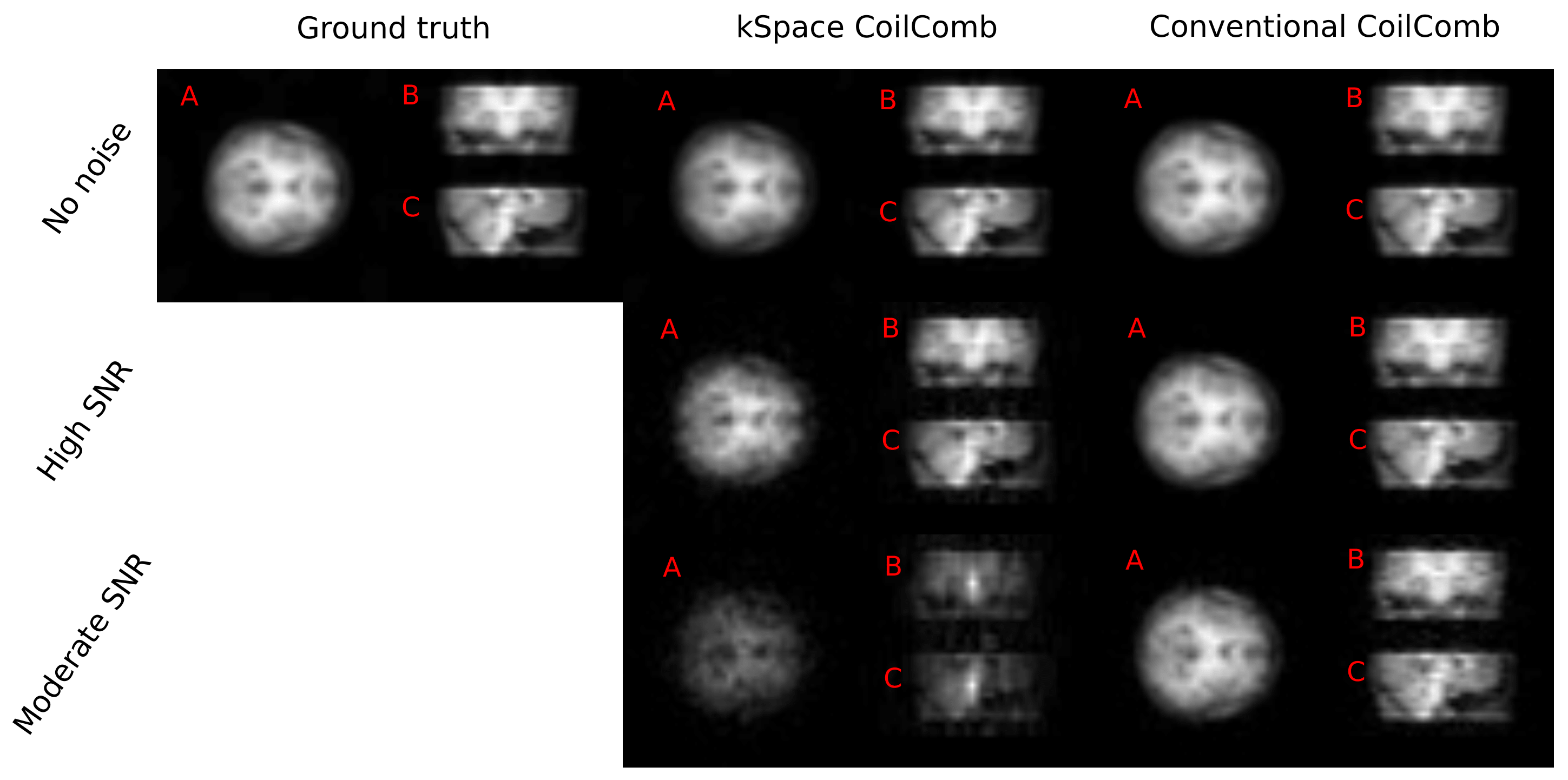
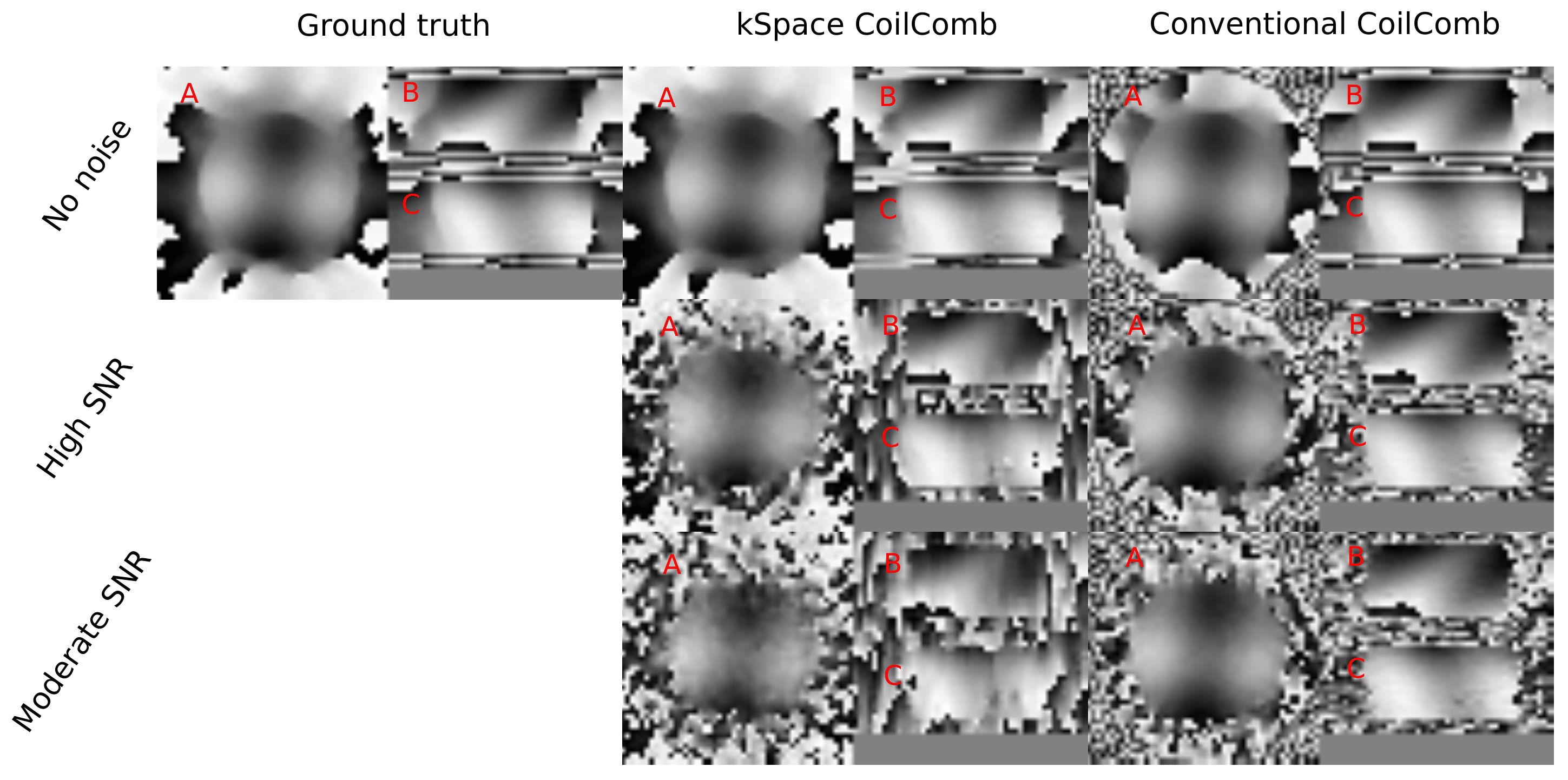
The non-Cartesian data were represented as a graph, where each kSpace location was a node connected by edges to the each node in Euclidean distance smaller than 1.5 FOV^-1. Each edge was weighted by the Euclidian distance. Real and imaginary parts of complex numbers were separated to independent features. The convolutional layer proposed by Kipf and Welling⁶ was used. As the validation data, small part of training data was used, which were not used in the training.Training parameters were: optimizer=Adam, Learning_rate=0.0001, loss=MSE, number_of_epochs=250, batch_size=10. The performance of the coil combination networks was evaluated on the validation data in cases of no noise scenario and in the presence of difference amount of noise.

RESULTS

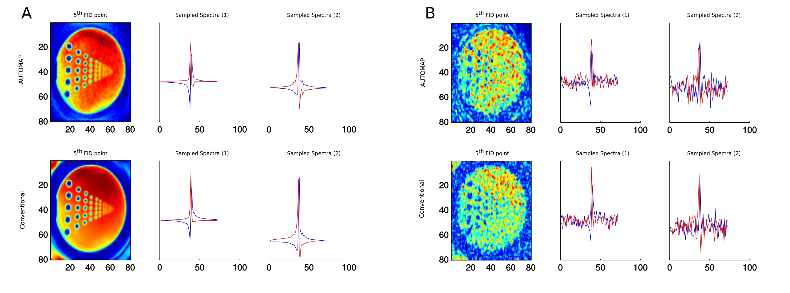
Results of AUTOMAP reconstruction of resolution phantom is shown in the first row of Fig.2. The second row of the Fig.2 depicts the results of conventional reconstruction. Results of kSpace coil combination is depicted in Fig.3 for magnitude images and in Fig.4 for phase images.

DISCUSSION and CONCLUSION

This abstract presents the preliminary results for replacing a standard MRSI reconstruction pipeline by deep learning approaches with the main goal to speed-up the whole reconstruction. AUTOMAP is capable of reconstructing MRSI data of the resolution phantom from non-Cartesian kSpace data even if each time point is reconstructed independently and the networks were trained on brain MRI. For high SNR data, spectra look very similar to conventional reconstruction. Due to its architecture, the multichannel data can’t be directly inserted as the input to the AUTOMAP reconstruction. Therefore, to complement our reconstruction strategy, the coil combination in kSpace domain on non-Cartesian points is required. The kSpace coil combination together with AUTOMAP will accelerate the MRSI reconstruction by ~2-3 orders of magnitude. From the results presented in Fig.3 and Fig.4, in principle, such coil combination is possible, however currently not applicable due to remaining instabilities due to noise, which will be addressed in future work.

Acknowledgements

This study was supported by the Austrian Science Fund (FWF): P30701