2845
31P Magnetic Resonance Spectroscopy analyzed and quantified by Convolutional Neural Network (CNN)1Department of Radiology and Medical Informatics, University of Geneva, Geneva, Switzerland, 2Department of Vascular Surgery, Centre Hospitalier Universitaire Vaudois and University of Lausanne, Lausanne, Switzerland, 3Faculty of Science and Medicine, Section of Medicine, University of Fribourg, Fribourg, Switzerland
Synopsis
Phosphorus magnetic resonance spectroscopy imaging (31P-MRSI) allows the probing of biological compounds that hold fundamental cellular information. High resolution MRSI at 3T suffers from low signal-to-noise ratio (SNR) inherent to the nuclear low sensitivity. This is accentuated in the MRSI in comparison to unlocalized free induction decay (FID) where acquired volumes are smaller and consequently lower the SNR. Our Convolutional Neural Network (CNN) based algorithm perform efficient quantification of metabolite and is compared to last-square fitting algorithm. Our model was trained with a simulated dataset and tested with both simulated spectra and real spectra from 3D 31P-MRSI acquired in kidneys.
Introduction
Among nuclei measurable by NMR, phosphorus (31P) is the most noteworthy behind the proton nucleus (1H) for its in-vivo application [1]. Phosphorus magnetic resonance spectroscopy (MRS) is a unique tool for monitoring cellular metabolism [2, 3]. Current state-of-the-art methods for identi- cation relies on non-linear tting algorithms such as AMARES [4], LCModel [5], QUEST or SVD techniques [6]. Machine learning has proven to be e cient numerical analysis for spectra analysis, with its ability to identify patterns features in data [7]. Recently, deep-learning techniques of CNN are used to perform 1H-MRS analysis and have shown at least comparable results as the current tting model [8, 9, 10]. This work presents an optimized method based on CNN algorithm combined with realistic data simulation to train an algorithm capable of accurate metabolite concentration estimation from 31P-MRS data and ex-vivo 3D 31P-MRSI of kidneys.Methods
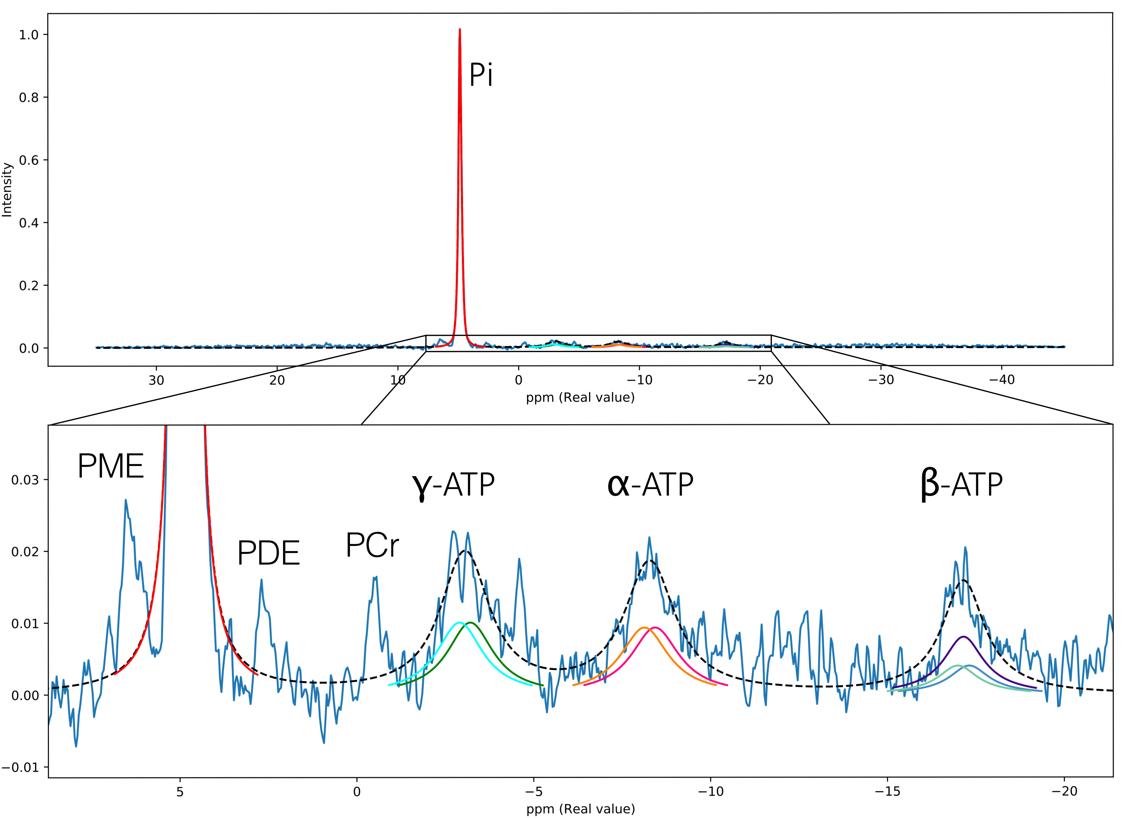
Metabolites of interest were selected: phosphocreatine (PCr), inorganic phosphate (Pi), adenosine triphosphate (α-ATP, β-ATP and γ-ATP), phosphomonoester (PME) including adenosine monophosphate (AMP), nicotinamide adenine dinucleotide (NAD+ and NADH) and phosphodiester (PDE). Simulated spectra contain 2048 points for a bandwidth of 4000 Hz, covering 80 ppm centered on the PCr frequency.First, spectra were quantified with a fitting method that is based on prior knowledge for spectral signature, peaks chemical shift and coupling constant. Once identified, the peaks are estimated with Gaussian shape curves, as illustrated in Figure 1.
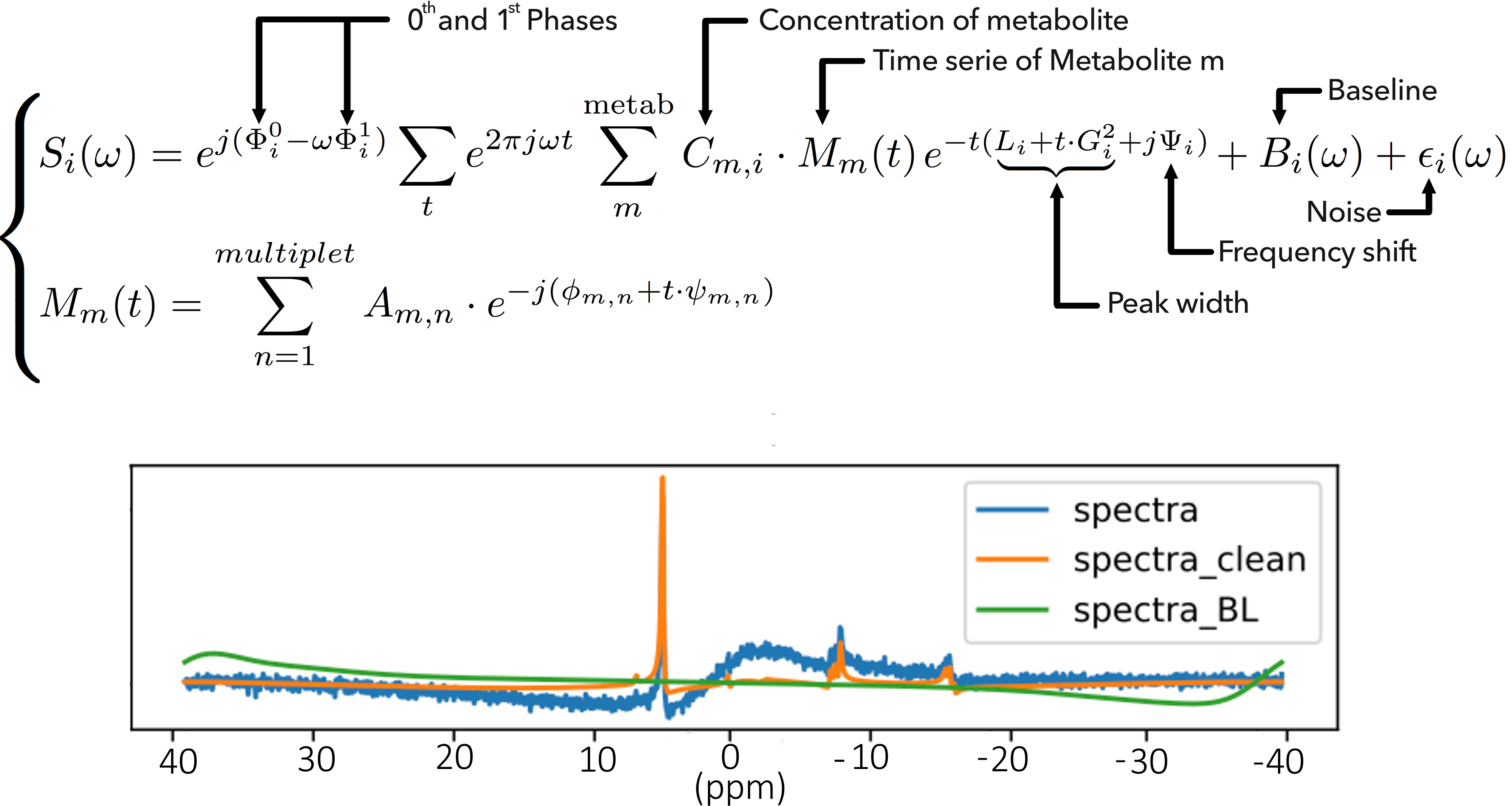
As second analysis, quantification was performed with the CNN. Supervised learning approach was achieved with a simulated and labeled training data-set. Following exact density matrix computation for each metabolite resonance, 106 spectra were generated with 33 independent variables, as shown on the Figure 2. The spectral parameters: concentration, zero and first order phase, frequency shift, peak width, white noise and added baseline were randomly determined for each specimen with normal distribution centered at the expected physiological values.
From the 106 spectra, 999000 of them were used for the training and 1000 for validation of the CNN, an other 1000 were used for testing. As a quality metric, the coefficient of determination R2 was used. The CNN received as input the complex values of the entire 31P spectrum and returns a multi-dimensional array that include the estimation of the metabolites concentration and the values of the parameters for each voxel.
Results
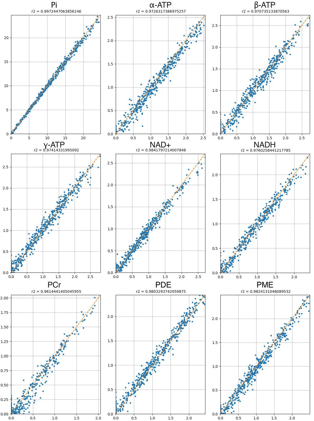
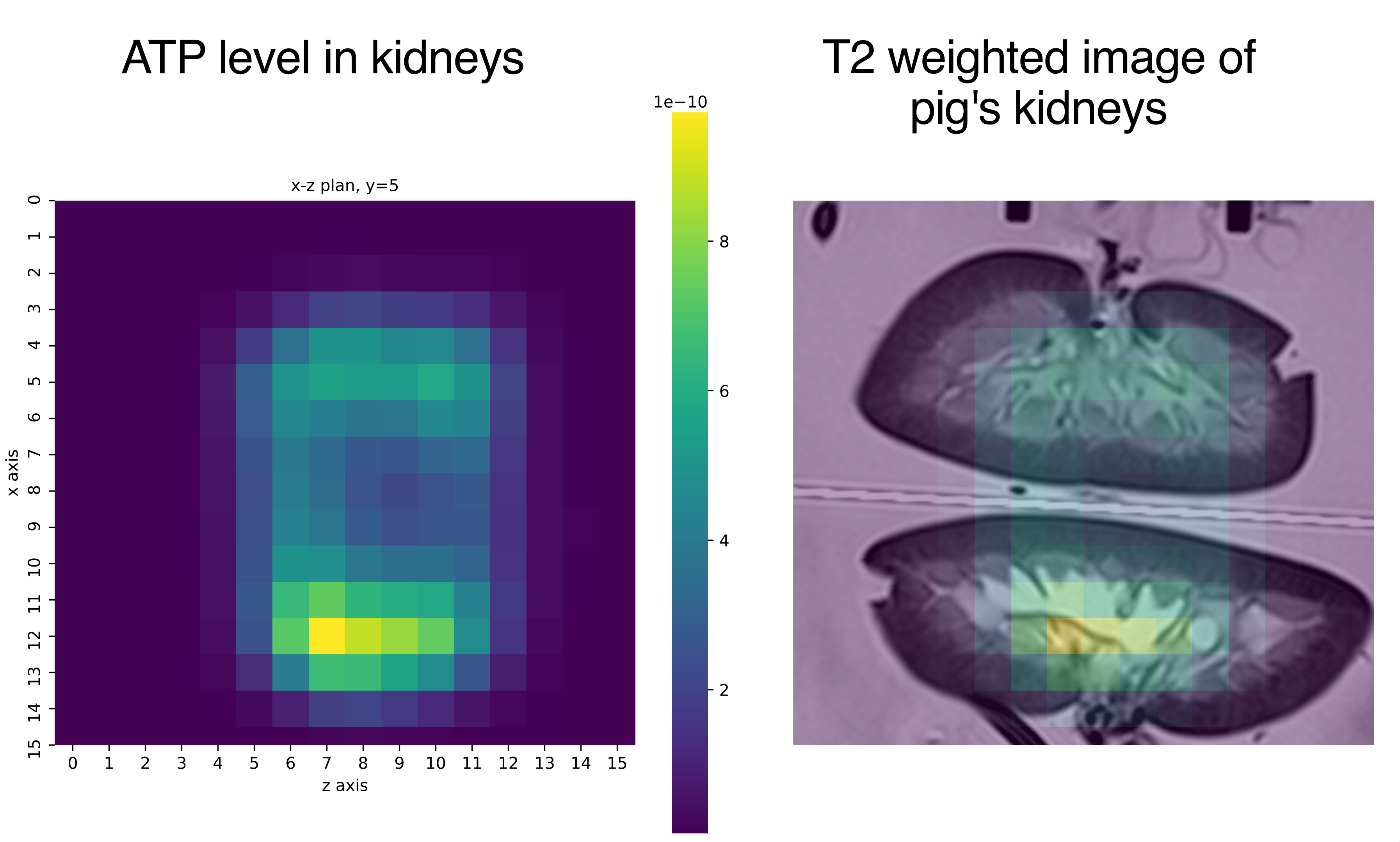
Figure 3 shows the coefficients of determination R2 for each metabolite. This evaluation is made on the testing data set, and it shows a very high ability to recover the values of the metabolite concentration as all values are above 0.96.Figure 4 shows a slice of a 3D 31P-CSI-MRS and its corresponding T2 image of pig's kidneys. The concentration map shows the ATP present in the kidney graft, as estimated by the fitting algorithm.
Discussion
The CNN shows encouraging preliminary results for MRSI spectra analysis. On test data-set, CNN is able to correctly estimate metabolite concentration. We aim to compare performance of the CNN with respect to the traditional fitting on the in-vivo data-set.The gain provided by the use of CNN is the instantaneous processing time in comparison with traditional fitting methods. Also the ability to create training set with widely distributed parameters should provide more robustness to CNN spectral analysis.
Acknowledgements
This study was supported by the Swiss National Foundation (No 320030_182658) and by the Center for Biomedical imaging (CIBM) of the Universities of Geneva and Lausanne, the University Hospitals of Geneva and Lausanne and the EPFL.References
[1] G. A. Webb, ed., Chapter 3 - Methods and Applications of Phosphorus NMR Spectroscopy In Vivo, vol. 75 of Annual Reports on NMR Spectroscopy. Academic Press, 2012.
[2] R. Buchli, D. Meier, E. Martin, and P. Boesiger, “Assessment of absolute metabolite concentrations in human tissue by 31p mrs in vivo. part ii: Muscle, liver, kidney,” Magnetic Resonance in Medicine 32 no. 4, (1994) 453–458.https://onlinelibrary.wiley.com/doi/abs/10.1002/mrm.1910320405.
[3] M. Chmelík, A. I. Schmid, S. Gruber, J. Szendroedi, M. Krššák, S. Trattnig, E. Moser, andM. Roden, “Three-dimensional high-resolution magnetic resonance spectroscopic imaging for absolute quanti cation of 31p metabolites in human liver,” Magnetic Resonance in Medicine 60no. 4, (2008) 796–802. https://onlinelibrary.wiley.com/doi/abs/10.1002/mrm.21762.
[4] L. Vanhamme, A. van den Boogaart, and S. V. Hu el, “Improved method for accurate and e cient quanti cation of mrs data with use of prior knowledge,” Journal of Magnetic Resonance 129 no. 1, (1997) 35 – 43.
[5] D. K. Deelchand, T.-M. Nguyen, X.-H. Zhu, F. Mochel, and P.-G. Henry, “Quanti cation of in vivo 31p nmr brain spectra using lcmodel,” NMR in Biomedicine 28 no. 6, (2015) 633–641.https://onlinelibrary.wiley.com/doi/abs/10.1002/nbm.3291.
[6] D. Graveron-Demilly, “Quanti cation in magnetic resonance spectroscopy based on semi-parametric approaches,” Magnetic Resonance Materials in Physics, Biology and Medicine27 no. 2, (Apr, 2014) 113–130. https://doi.org/10.1007/s10334-013-0393-4.
[7] S. S. Gurbani, S. Sheri , A. A. Maudsley, H. Shim, and L. A. Cooper, “Incorporation of a spectral model in a convolutional neural network for accelerated spectral tting,” Magnetic Resonance in Medicine 81 no. 5, (2019) 3346–3357.https://onlinelibrary.wiley.com/doi/abs/10.1002/mrm.27641.
[8] S. Courvoisier, A. Klauser, and F. Lazeyras, “High-resolution magnetic resonance spectroscopic imaging quanti cation by convolutional neural network,” ISMRM abstract (2019).
[9] N. Hatami, M. Sdika, and H. Ratiney, “Magnetic resonance spectroscopy quanti cation using deep learning,” in Medical Image Computing and Computer Assisted Intervention – MICCAI 2018, A. F. Frangi, J. A. Schnabel, C. Davatzikos, C. Alberola-López, and G. Fichtinger, eds., pp. 467–475. Springer International Publishing, Cham, 2018.
[10] D. Das, E. Coello, R. F. Schulte, and B. H. Menze, “Quanti cation of metabolites in magnetic resonance spectroscopic imaging using machine learning,” in Medical Image Computing and Computer Assisted Intervention − MICCAI 2017, M. Descoteaux, L. Maier-Hein, A. Franz,P. Jannin, D. L. Collins, and S. Duchesne, eds., pp. 462–470. Springer International Publishing, Cham, 2017.
Figures