Purpose

Recently, it has been shown that a convolution neuronal network (CNN) can be used to quantify metabolites in magnetic resonance spectroscopy (MRS)^1,4. The network is designed to suppress noise, reduce linewidth and remove baseline that usually hampers the reliability of the quantification of metabolites. After CNN, intact metabolite spectra can be directly deconvoluted with simulated spectra from basis sets for quantities of multiple metabolites. In this implementation, metabolites concentrations were estimated in a relative way because signal input into CNN was normalized during calculation. Therefore, the concentrations from CNN can be compared between subjects/scans using relative quantification such as ratio to creatine (Cre). In MRS, the level of signal intensity is necessary for performing water scaling so that metabolite signal can be calibrated to the institutional unit for between subject comparison. In this study, a CNN is constructed using simulated spectra¹ and we investigate the variation of quantified metabolites at various signal levels of the input signal. We also propose a strategy to perform scaling for the input data using water signal so that metabolite concentrations can be reported in institutional units for general use.

Methods

The CNN structure includes 3 convolution blocks, 2 max pooling layer between convolution block and a fully connected layer. For each convolution blocks, it contains convolution, batch normalization and activation layer for 4 repetitions. Data preprocessing and model implementation are using Python 3.6, Keras 2.2.4 with tensorflow 1.13.1. We simulated 50000 spectra using basis sets from LCModel (3T PRESS TE30), which contains 15 metabolites. Concentrations were varied with different levels of noise, macromolecules (MM), line broaden using the same setting as previous study^1,2. The CNN was trained with 40000 training data, 5000 validation data and 5000 test data with SGDM optimizer and MSE loss function. In vivo MRS data were collected on 2 healthy subjects on 3T Siemens Skyra system (Siemens, Emlargen, German) using PRESS sequence (TR/TE:2000/30 ms, sample points:2048, bandwidth:2000 Hz, NEX:64). MRS data were collected at dorsal lateral prefrontal cortex (DLPFC) and primary motor area (M1). The same protocol was repeated 5 times in three days with non water suppression (NWS) spectra acquired using the same parameters for each subject. Before entering CNN, in vivo spectra were multiplied by different scaling factors. The output spectra of CNN were quantified using deconvolution method¹ for each metabolite and quantified metabolites were normalized using concentrations denoted by LCModel basis. In vivo spectra were also quantified using LCModel with water scaling. The repeatability of quantified concentrations was evaluated using the coefficient of variance (COV). The proposed scaling factor (W_ratio) for input ³ was calculated as the ratio of water signal of simulated spectra and in vivo water signal, which stands for the signal gain between simulated spectra and in vivo spectra. The water signal of simulated spectra is calculated according to the concentrations denoted for each metabolite in the basis set by assuming the water concentrations to 55.55 M and in vivo water signal is NWS spectra. The scaling factor of 1, 200, 500, 1000, and W_ratio were applied, respectively, and the quantified metabolite concentrations were compared to those from LCModel.

Results

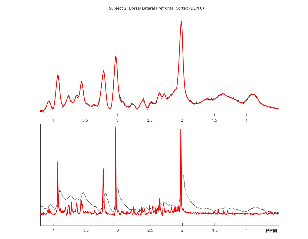
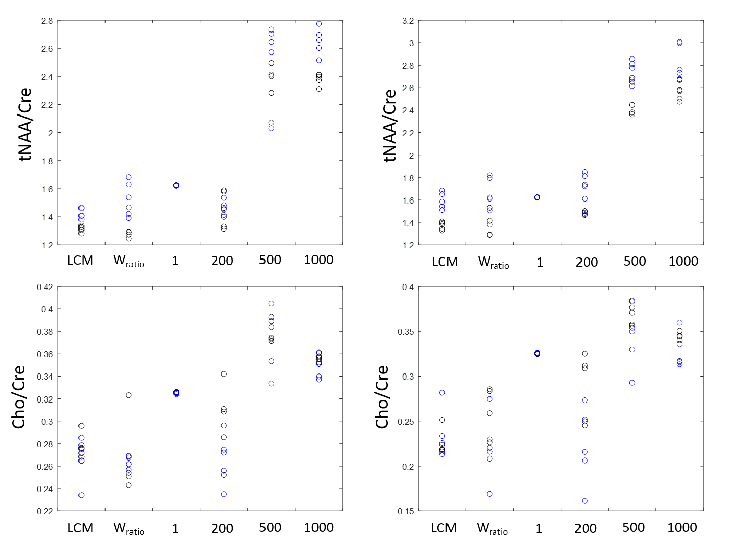
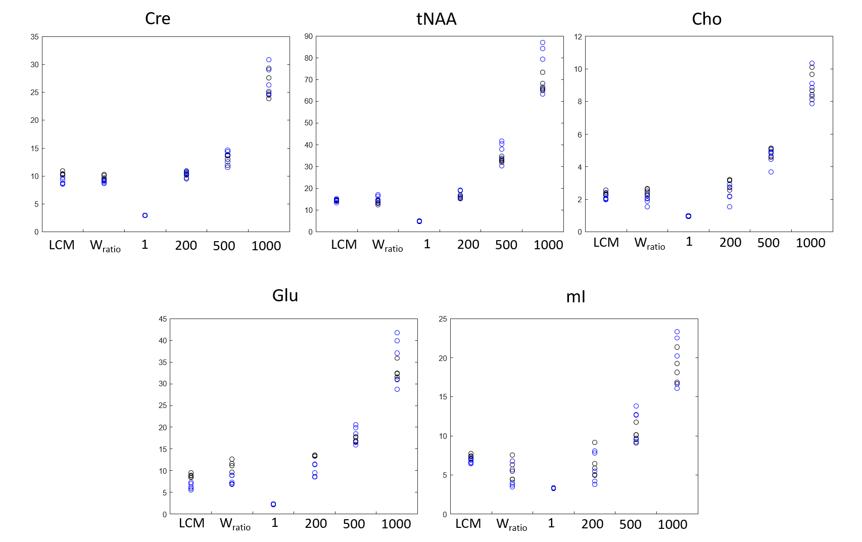
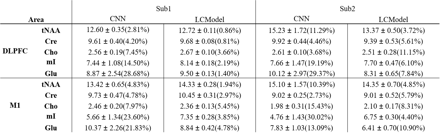
Figure 1 shows the spectra of DLPFC output by CNN and fitted by LCModel. Figure 2 showed the relative concentration of tNAA and Cho (ratio to Cre) from LCModel and CNN, where the W_ratio varied from 150.0 to 248.4. For both region, using the scaling factor of W_ratio gives similar results to LCModel in terms of level and variations. Figure 3 shows the concentrations of Cre, tNAA, Cho, Glu and mI from LCModel and CNN using different scaling factor. We can see that quantified concentrations are similar to LCModel using W_ratio as scaling factor and the concentrations merge to upper and lower bound of simulated spectra at a large to small scaling factor. Table 1 summarized the mean, standard deviation and COV of tNAA, Cre, Cho, mI and Glu in 5 repeated scans. For both regions, consistent metabolite levels were found in CNN and LCModel but with larger COV in CNN than LCModel especially for Glu and mI.

Discussion and Conclusions

In this study, we showed that using water signal as a scaling factor can properly scale the output of CNN so that the quantified concentrations can be comparable to those from LCModel (Table 1). When the signal level of input spectra is lower or higher than the simulated spectra using to train the CNN, the quantified metabolite may be trapped to upper and lower bound of the simulated concentration (Figure 3), which yields variation in the relative quantification of concentrations (Figure 2). We further find that with proper scaling factor as the proposed water signal scaling strategy, the output of CNN can be quantified using a commonly used water scaling method (Figure 3). However, the quantification of CNN shows lower repeatability (higher COV) than LCModel. In conclusion, we have proposed a strategy to quantify CNN output spectra in an institutional unit. Although the results are comparable to conventional LCModel results, a further study is necessary to validate this method using phantom and theoretical model should be established with further understanding of the CNN model.

Acknowledgements

This study was supported in part by grants from the Ministry of Science and Technology (MOST 108-2314-B-004 -001 -MY3 and MOST 108-2221-E-011 -117 -MY3). The authors thank Taiwan Brain and Mind Imaging Center (TMBIC) and National Cheng-Chi University for consultation and instrument availability for this work.