Purpose:

Recent progress in convolutional neural networks (CNN)^1,2 and processing power has provided new tools for signal processing. Magnetic Resonance Spectroscopy (MRS) is a powerful quantitative tool, which allows access notably to lipid composition in the brain, liver, muscle, subcutaneous adipose tissue, and bone marrow. Quantification of MRS is based on modelling of the MRS signal (in the time or frequency domain). However, depending on the fat fraction (FF) in the MRS spectrum, the method of quantification and model used for the lipid composition vary³. Recent studies have proposed the use of a simplified model with a reduced number of parameters describing an average composition of triglycerides to estimate (CL: chain length, nmidb: number of middle interrupted double bound, ndb: number of double bound)⁴. CNNs are independent of any priors and are solely dependent on the number of signals used for training hence, are model agnostic. To our knowledge, few CNNs have been designed for MRS signal quantification⁵ and in particular for lipid signal quantification. Therefore, we aim to design and evaluate a NN for lipid MRS quantification using simulated data.

Methodology

Data Simulation: Simulated data were obtained using SPINACH 2.4 spin dynamics simulation library6 (STEAM sequence, B0 = 3T, nPts = 2048, sampling frequency = 4000Hz) for averaged fatty acids signal for value of ndb = 0.1 to 5, nmidb = 0.001 to 1.85 and CL = 16.825 to 18.05 and a water signal was added to have a FF = 2 to 90 %. Components of the fatty acids and water signal were T2-weighted according to values of the literature and 6 levels of Gaussian white noise were added (standard deviation = 0 to 10 % of the maximum value).
Network Design: Different convolutional neural networks were trained using time-domain simulated signals to predict FF, CL, ndb and nmidb using a varying number of layers (short : 4,medium: 7 and long: 13) and training loss functions ( MSE: mean squared error, MAE: mean absolute error, MAPE: mean absolute percentage error).
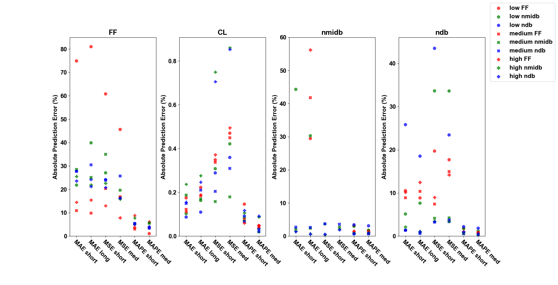
Network Training: Dataset was split into a training set with 30k signal, a validation set of 5k signal and a test set of 3.7k signals. Stopping criteria for the training was based on the value of validation loss after a period of 50 iterations, learning rate has been chosen empirically and a batch size of 128 was used for training the CNN. The training was made on Tensorflow 1.13.1 using two 16GB Tesla V-100 GPUs and takes approx. from 3 days 1 hour 30 minutes to 5 days 6 hours 47 minutes depending on the CNN trained. Network evaluation: Assessment of correlation between predicted values and test data ground truth-values were used to evaluate the CNN performance. The test data is divided into sets with low level FF ( 2-20 %), medium level FF (20-60 %) ,high level FF (60-90 %), low level nmidb (0.001-0.611),medium level nmidb (0.611-1.221), high level nmidb (1.221-1.85), low level ndb (0.1-2), medium level ndb (2-4) and high level ndb (4-5). The percentage absolute error between predicted and true parameters was used as a metric to evaluate the effectiveness of CNN’s predictions.

Results

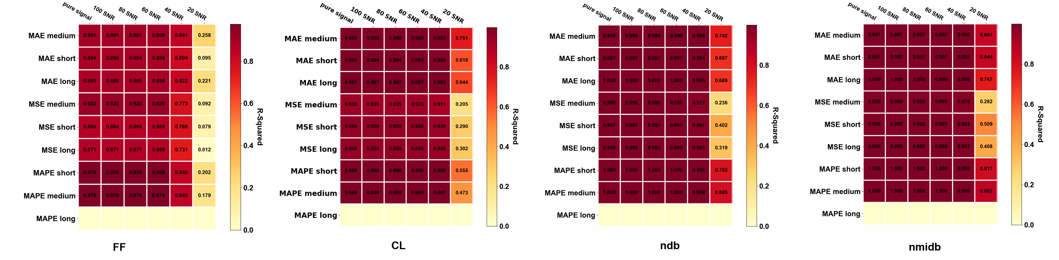
Table 1 shows the CNN architectures evaluated. Figure 1 shows that medium depth CNN architecture (number of layers =7, number of trainable parameters=4,124) using MAPE as the training loss function gives the best performance. The parameters predicted by the CNN model gives the best correlation with true values (average R-squared statistics FF= 0.828, CL = 0.908, ndb = 0.976, nmidb = 0.966). Figure 2 reafirms the conclusion of figure 1, it shows that the absolute prediction error (%) for the CNN is less than 10% for all parameters across all sets of test data (FF = 1.1% -7%, CL = 0.01 - 0.07 %, nmidb = 0.6 - 2.6 %, ndb = 0.23 -1.34 %).

Conclusion

Nonlinear regression using CNN is a viable tool to quantify lipid composition in MRS lipid time-domain signals. The 7-layer architecture is the best CNN architecture for MRS quantification and an increase or decrease in layer number does not change the effectiveness of the neural network. MAPE provides for a CNN network with maximum accuracy and the network trained using the loss function is robust to variability within the dataset and prediction accuracy is high for all Fat composition parameters. In the future expanding on the experiment, we aim (i) to evaluate the effectiveness of CNNs on in vivo MRS lipid signals; (ii) to train the CNNs based MRS quantification to account for inhomogeneity in magnetic field and eddy effect during MRS acquisition; (iii) design neural network architectures that best quantify MRS lipid signal in frequency-domain and compare them with the CNNs used for time-domain signals.

Acknowledgements

No acknowledgement found.