Introduction

Quantitative R_1ρ dispersion could provide a unique structural information on collagen integrity in cartilage.¹ Substantial artifacts could arise from non-uniform B₀ and B₁ fields in varying R_1ρ-weighted images, particularly at higher B₀ with an extreme spin-lock (SL) RF strength (ω₁/2π).^2-4 Recently, a few self-compensated SL methods have been developed; however, none of these existing approaches would be robust enough for a wide range of ω₁/2π.⁵ Hence, this work aimed to introduce a new SL scheme for quantitative R_1ρ dispersion in cartilage.

Methods

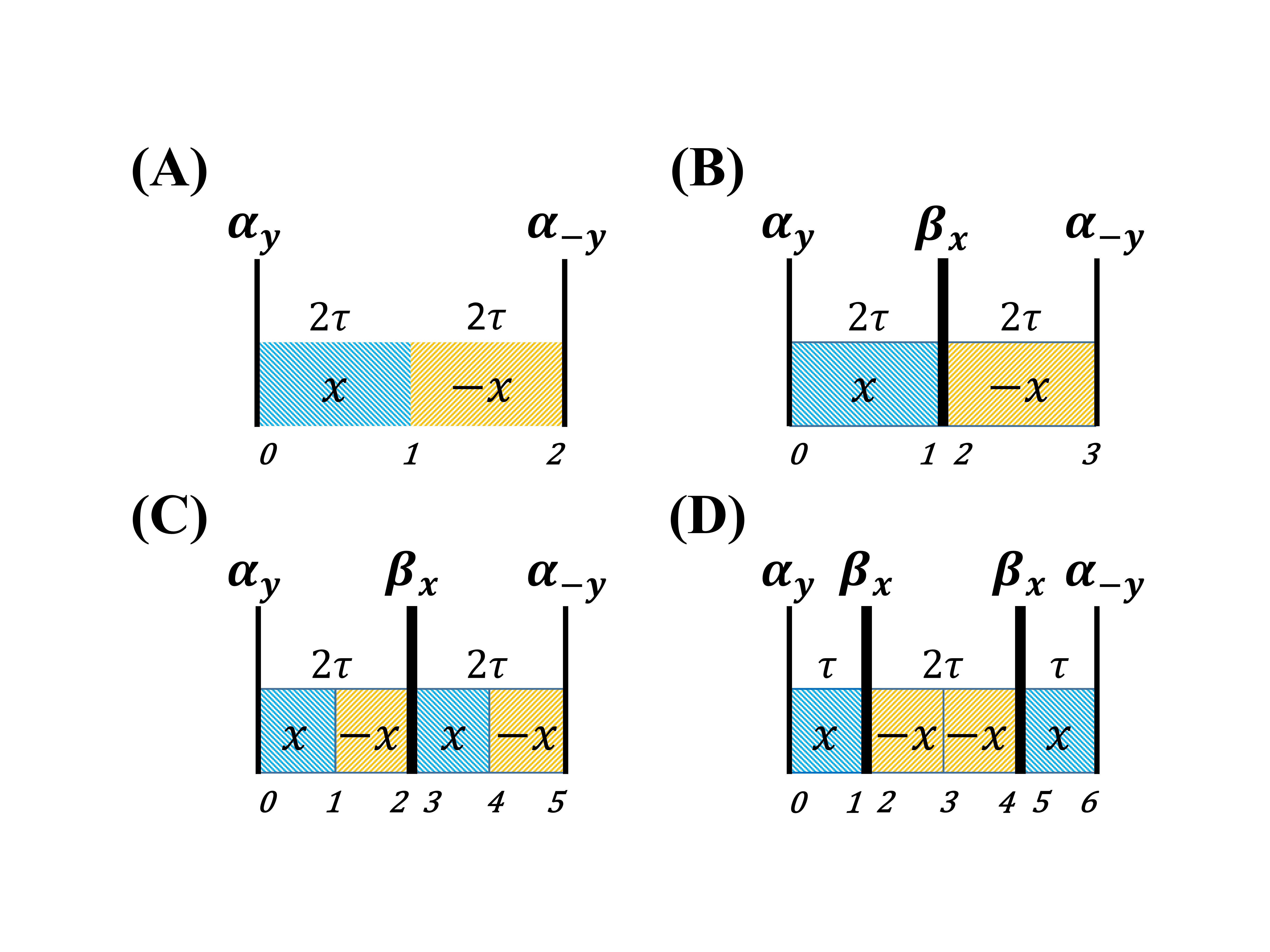
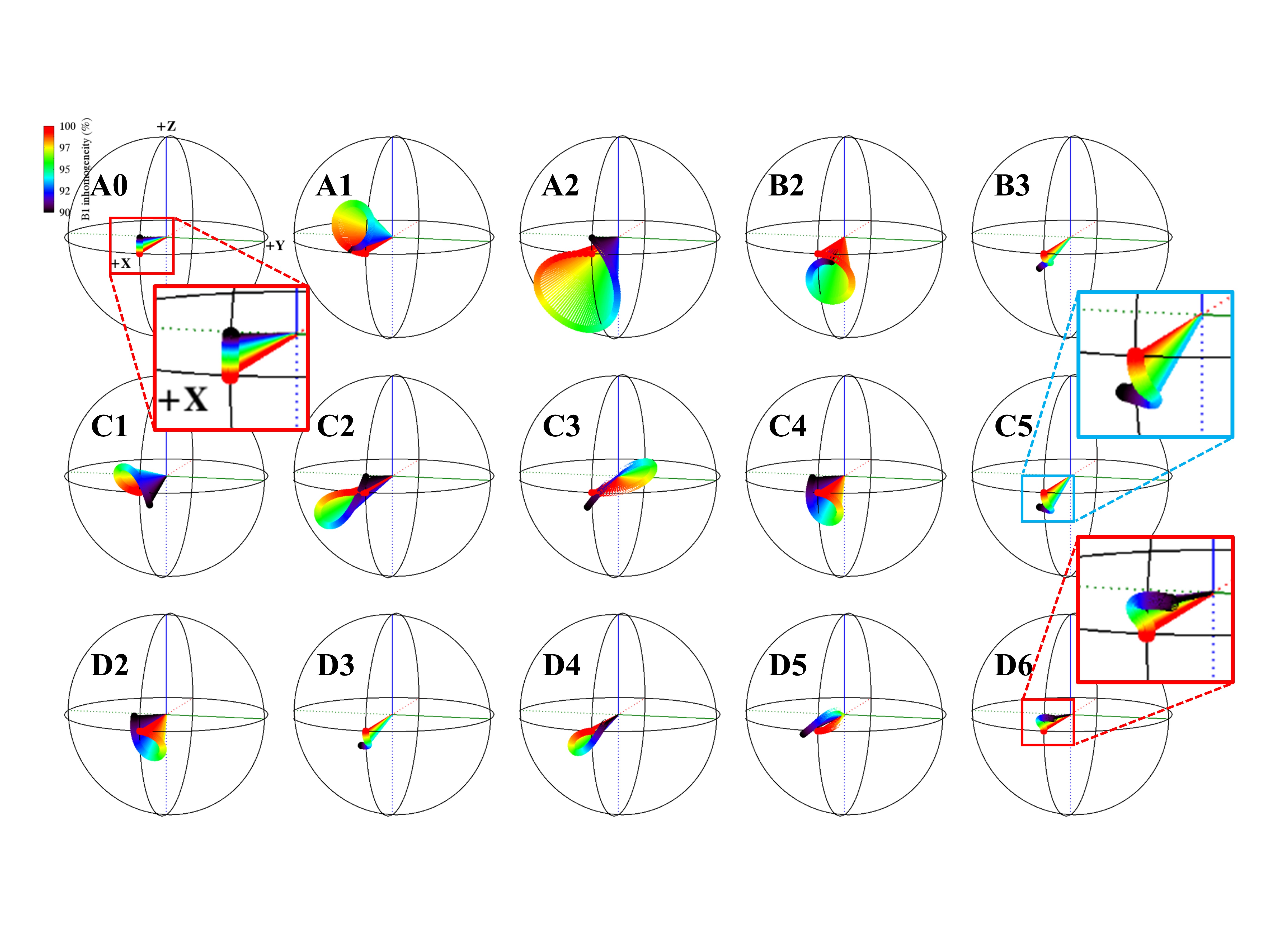
(1) Spin-locking schemes: Figure 1 sketches the reported (A-C)^2-4 and the proposed (D) SL schemes. The digital numbers under these sketches indicate the specific time points on which the simulated spin trajectories will be visualized. (2) Spin dynamics simulations: A spin dynamics was simulated for 4 SL schemes with ω₁/2π progressively increased from 0 to 1000 Hz in 101 steps and likewise with Δω₀/2π from 0 to 250 Hz. The nominal FA α and β were scaled down 90% to mimic B₁ inhomogeneity. (3) Spin trajectory visualizations: Some simulations were highlighted with an ensemble of 101 spins that were respectively exposed to a nominal ω₁/2π of 500 Hz with B₁ homogeneity progressively improved from 90% to 100% of the nominal value, and to a progressively increased Δω₀/2π from 0 to 250 Hz. The spin dynamics were visualized in Figure 3 as follows: A0 -> A1 -> A2 (A); A0 -> A1 -> B2 -> B3 (B); A0 -> C1 -> C2 -> C3 -> C4 -> C5 (C) and A0 -> C1 -> D2 -> D3 -> D4 -> D5 -> D6 (D). (4) MR imaging protocol: R_1ρ-prepared signals using 4 SL schemes were imaged by 3D TFE following an elliptical centric phase-encoding (low-high) order on a 3T scanner using a 16-ch T/R knee coil. Other parameters: ω₁/2π=50, 125, 250, 500, 750, 1000 Hz; shot interval = 2 s; TFE factor = 64; TR/TE = 5.4/2.8 ms; FA = 10° ; voxel size = 1.0*1.0*3.0 mm³; CS-SENSE factor = 2.5; acquisition duration = 40 s per 3D R_1ρ-weighted image scan. B₀ and B₁ fields were mapped on phantom using conventional dual-echo ( ΔTE of 3 ms) and dual-TR (TR=30 and 150 ms) methods. (5) R_1ρ dispersion modeling: A voxel intensity S (in a logarithmic scale) in R_1ρ-weighted image of cartilage at 3T could be expressed using the following Eq.,
$$ ln(S) = P-R_{2a}/(1+4ω_1^2τ_b^2) $$
where P stood for $$$ln(S_0)/TSL-R_{2i}$$$, S₀ and TSL (=40 ms) were constant, R_2i and R_2a were two predominant contributions to R₂, and ω₁ and τ_b were a SL RF power and an effective “slow” correlation time.¹ A sum of squared errors (SSE) was used to assess the discrepancies between the measured and the modeled data in vivo. When R_1ρ dispersion was not expected for agarose (1-4%, w/v) gels,⁶ their signal fluctuations were quantified with coefficients of variation CVs (%) as ω₁ altered. All data analysis and visualization were carried out with a customized software developed in IDL 8.5 (Harris Geospatial Solutions, Inc, Boulder, CO).

Results and Discussion

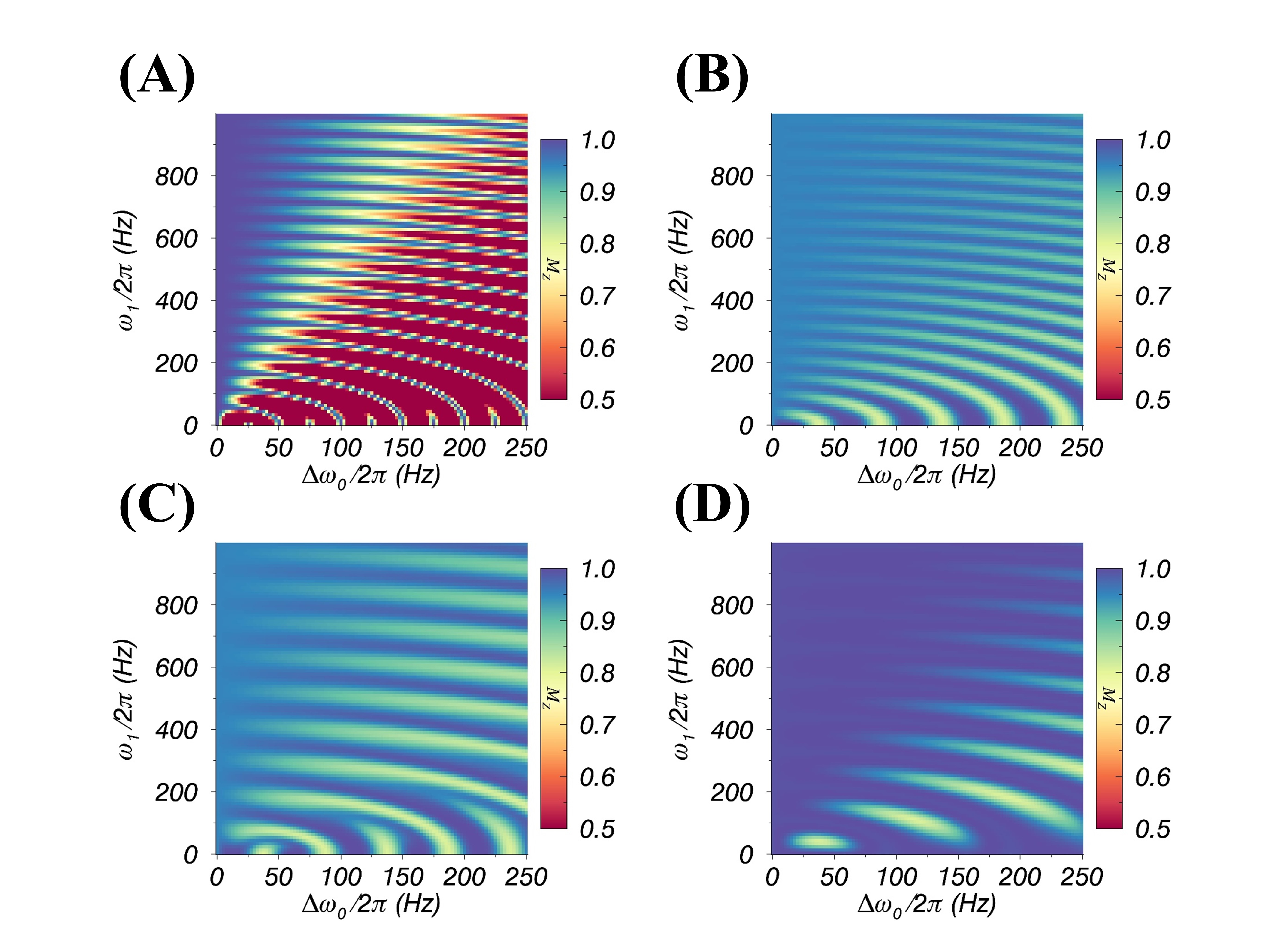
Figure 2 presents the simulated longitudinal magnetizations. Compared with the reported methods A-C, the proposed scheme D demonstrated markedly reduced sensitivity to ΔB₀ and ΔB₁. This finding could be visualized on Bloch spheres as shown in Figure 3, where the resulting spin trajectories just before α_-y pulse were represented in A2, B3, C5 and D6, indicating that the least and most close trajectories with respect to A0 were A2 and D6, respectively. In other words, the scheme D could offer not only a relatively higher tolerance to ΔB₀ and ΔB₁, but also a lesser signal loss. Figure 4A-D show one exemplary R_1ρ-weighted image slice of phantom. Qualitatively, the scheme D demonstrated fewer banding artifacts, particularly when using a lower ω₁/2π. Figure 4E presents quantitatively that the method D (filled black circle) provided the least signal fluctuations with the smallest average CV (%), based on the measurements from 2 ROIs located inside and outside agarose tubes. ΔB₀ (ppm) and B₁ (%) field maps for the same image slice are respectively shown in Figure 4F and 4G. The observed B₁ field was very close to its normal value (i.e. ~100%); however, the measured ΔB₀ was markedly varied as much as more than 1 ppm (i.e. >128 Hz) near the interfaces in which the banding artifacts became more prominent. Figure 5 demonstrates one exemplary R_1ρ-weighted image slice of human knee. The image banding artifacts could barely be recognized except the image acquired with the scheme A using ω₁/2π of 125 Hz. Two exemplary signal intensities were derived from 2 ROIs located on the posterior tibial (PTC) and the central femoral (CFC) cartilage. The measured and fitted R_1ρ dispersion profiles were compared in the 3^rd row. The observed SSE (*10^-3) for SL schemes A-D were respectively 1.2, 0.4, 0.1, and 0.3 for CFC (blue lines). In comparison, those values were 7.2, 3.2, 2.8, and 0.4, for PTC (red lines). These fitting results suggest that the proposed SL scheme D could improve R_1ρ dispersion quantification accuracy of human knee cartilage.

Conclusion

In conclusion, a robust spin-locking scheme has been developed for quantitative R_1ρ dispersion on human knee cartilage.

Acknowledgements

This work was supported in part by the Eunice Kennedy Shriver National Institute of Child Health & Human Development of the National Institutes of Health under Award Number R01HD093626 (Prof. Riann Palmieri-Smith). The content is solely the responsibility of the author and does not necessarily represent the official views of the National Institutes of Health. The author would also like to thank Prof. Thomas Chenevert for his support and encouragement, and Suzan Lowe and James O’Connor for their assistance in collecting human knee images.