Introduction

Ultrashort Echo-Time (UTE) imaging techniques that can visualize short T₂* components are investigated for many applications, such as bone imaging, transcranial MR-guided focused ultrasound treatment, CT image synthesis, and PET attenuation correction^1-4. For these applications, multi-echo UTE is used to visualize the bone images by subtraction or division of short and long TE images, or by conventional mapping^2-3,5. However, these methods may have low accuracy in the regions composed of low-density bone or bone marrow. In this study, we propose the hyperbolic tangent based R₂* model. The hyperbolic tangent based R2* model is suggested to separate the bone and soft tissue in human head and the utility of the proposed method is verified by evaluating the bone and soft tissue segmented R₂* contrast maps with various TE.

Methods

1. Hyperbolic Tangent based R₂* Model

The magnitude only water-fat signal equation can be expressed as:
$$
{|S_i|}^2={{W^2+F^2+2WFcos(2\pi\Delta f \cdot {TE}_i)}}e^{-2R_2^* \cdot {TE}_i}
$$
where the $$$S_{i}$$$ is the measured data at $$$i_{th}$$$ TE ($$${TE}_{i}$$$), $$$W$$$ and $$$F$$$ denote signals from water and fat, respectively. $$$\Delta f$$$ is the water-fat frequency shift for single spectral peak model and the relaxation rate $$$R_{2}^*$$$ is the reciprocal of relaxation time $$$T_{2}^*$$$. Then the ratio of the difference and sum of $$${|S_i|}^2$$$ and $$${|S_{in}|}^2$$$ ($$${|S_{in}|}$$$ is measured signal at in-phase TE) is given by:
$$
\frac{{|S_{i}|}^2-{|S_{in}|}^2}{{|S_{i}|}^2+{|S_{in}|}^2}=\frac{{(W+F)^2{sinh(R_2 ^*\cdot(TE_{in}-TE_{i}))}-2WF{sin}^2(\pi \Delta f \cdot {TE}_i)}e^{-2R_2^* \cdot({TE}_{in}-{TE}_{i})}}{{(W+F)^2{cosh(R_2 ^*\cdot(TE_{in}-TE_{i}))}-2WF{sin}^2(\pi \Delta f \cdot {TE}_i)}e^{-2R_2^* \cdot({TE}_{in}-{TE}_{i})}}
$$
Let $$$sinh(R_2 ^*\cdot(TE_{in}-TE_{i}))=HS$$$, $$$cosh(R_2 ^*\cdot(TE_{in}-TE_{i}))=HC$$$, and $$${sin}^2(\pi \Delta f \cdot {TE}_i)e^{-2R_2^* \cdot({TE}_{in}-{TE}_{i})}=SS$$$. Under the condition 1 for $$$HS>>SS$$$ and condition 2 for $$$HC>>SS$$$, the ratio $$$\frac{{|S_{i}|}^2-{|S_{in}|}^2}{{|S_{i}|}^2+{|S_{in}|}^2}$$$ can be approximated as:
$$
\frac{{|S_{i}|}^2-{|S_{in}|}^2}{{|S_{i}|}^2+{|S_{in}|}^2} \approx tanh(R_{2}^*\cdot \Delta {TE}_{i}),
$$
$$
where \Delta {TE}_{i}=TE_{in}-TE_{i}
$$
which gives the same procedure for calculating $$$R_2^*$$$ values. If the data sets are against to those conditions, incorrect R₂* values will be computed in tissues which are composed of both water and fat (i.e., bone marrow).

2. Decomposition of High and Low $$$R_2^*$$$ Components

To separate the bone and soft tissue components, small quantity approximation $$$(tanh(x)=x)$$$ was used. Because R₂* of bone is much higher than that of soft tissue, subtracting the maximum value that satisfied $$$tanh(R_2^* \cdot \Delta {TE}_i)=R_2^* \cdot \Delta {TE}_i$$$ from the $$$tanh(R_2^* \cdot \Delta {TE}_i)$$$ over the volume makes the subtracted values of bone and soft tissue to positive and negative, respectively. Finally, square roots of those can be decomposed to real and imaginary components as bone and soft tissue.

3. MRI Data Acquisition and Processing

Two sequences on a 3.0 T MRI scanner was used: Dual-echo UTE (Philips Achieva, The Netherlands) and ZTE (GE Signa Architect, Milwaukee, WI). MR Images were acquired with the following parameters: (UTE= TE1:0.15/0.25/0.35/0.45/0.55ms, TE2:2.3ms, TR:5.3ms, field-of-view:24$$$\times$$$24$$$\times$$$24cm³, flip angle:$$$5^{\circ}$$$, acquisition density of angles:80%, 1.5mm isotropic resolution, scan time:3’37’’/ ZTE= TR:533.5ms, field-of-view:26$$$\times$$$26$$$\times$$$26cm³, flip angle:$$$1^{\circ}$$$, voxel size:1$$$\times$$$1$$$\times$$$1mm³, scan time:4’2’’). Inverse logarithmic ZTE images were calculated to compare the structure of bone with the proposed method using UTE imaging⁶. Registration of UTE and ZTE images is performed using 3D Slicer⁷.

Results

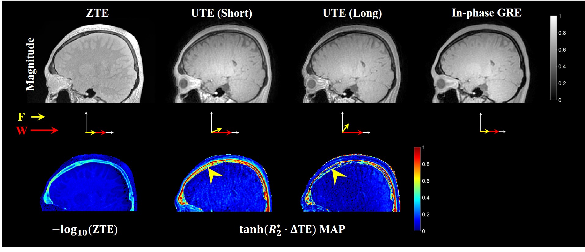
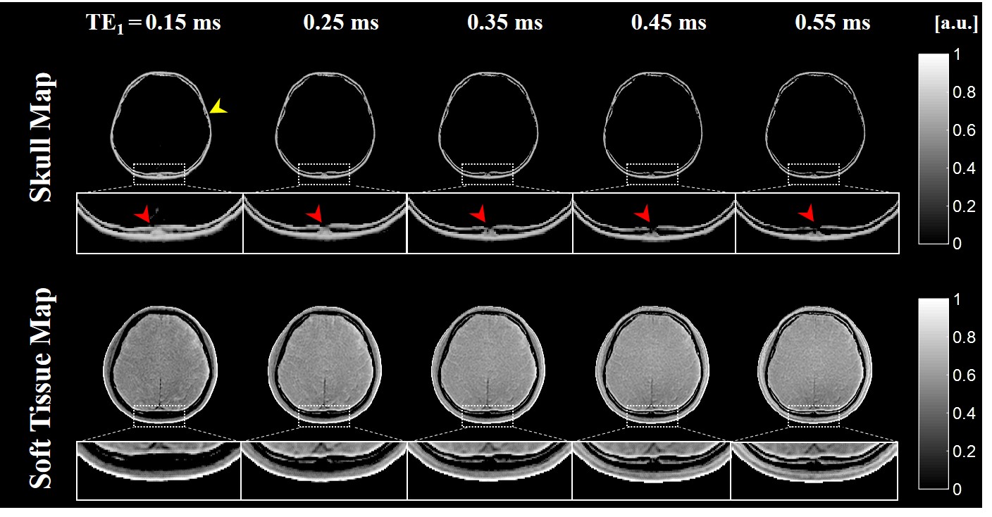
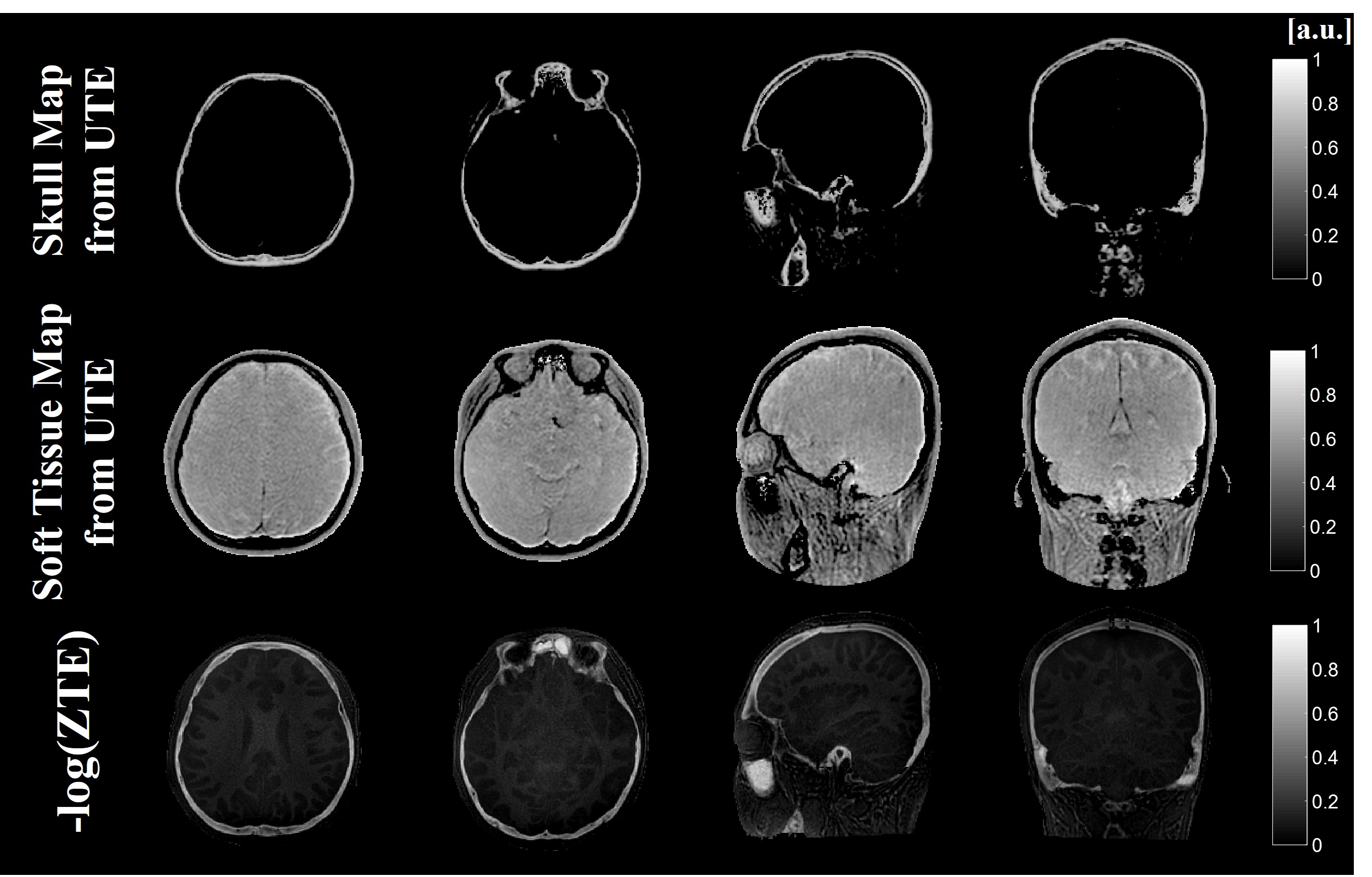
A set of ZTE, UTE and in-phase GRE magnitude images of the head is shown in Fig. 1. Since the long TE₁ cannot satisfy the condition 1 and 2, $$$tanh(R_{2}^*\cdot \Delta {TE}_{i})$$$ map from dual-echo UTE images show that the skull is decomposed imperfectly, especially in bone marrow region (Fig. 1). Compared with the -log(ZTE), $$$tanh(R_{2}^*\cdot \Delta {TE}_{i})$$$ obtained from dual-echo UTE images shows much higher difference between bone marrow and soft tissue. The reconstructed skull and soft tissue maps along five different TE₁ are shown in Fig. 2. Bone marrow regions are reconstructed in soft tissue map increasingly when TE₁ increases. Comparing the skull map reconstructed from images of shortest TE to the inverse logarithmic ZTE, skull layers are shown to be well depicted in Fig. 3.

Discussion and Conclusions

We proposed the hyperbolic tangent based R₂^* model using dual-echo UTE imaging. The results demonstrated that the cortical bone, trabecular bone, bone marrow, and soft tissue are well-segmented by using the proposed hyperbolic tangent based R₂^* model. In contrast with the inverse logarithmic ZTE map, bone marrow is well decomposed from the skull map in the proposed method. In conclusion, For the applications which should consider both cortical bone and bone marrow, such as MR-only transcranial focused ultrasound treatment planning, hyperbolic tangent model using UTE image can provide the whole structures in skull without missing layers.

Acknowledgements

This work was supported by the Technology Innovation Program (#10076675) funded by the Ministry of Trade, Industry Energy (MOTIE, Korea).