INTRODUCTION

Renal MRI has undergone significant developments in recent years, but standardisation and multicentre evaluation of measures is now crucial for clinical translation [1]. The UK Renal Imaging Network - MRI Acquisition and Processing Standardisation (UKRIN-MAPS) framework [2] aims to develop harmonized renal MRI protocols across MR vendors. This abstract presents initial results for measures of renal T₁ and BOLD T₂*, and characterization of scanner variability from B₀ and B₁ field maps.

METHODS

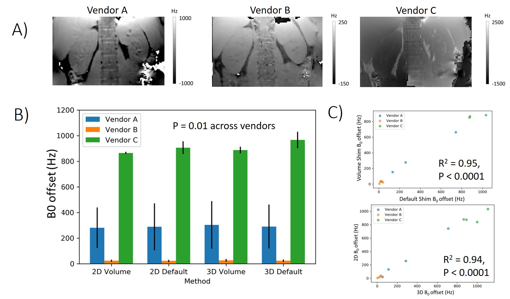
Data Acquisition: Data was collected on four healthy subjects (age 33±8 years) at three UK sites each with a 3T scanner from a different MR vendor (GE, Siemens, Philips). Median time between scans of the same subject in each vendor was 24 days. The data was acquired using predominantly product sequences with near-identical acquisition parameters across vendors. All relaxometry data was collected with a 384x384x5mm² FOV and 3x3x5mm³ voxel resolution.
B₀ field map: Dual-echo gradient echo scheme (echo shift ΔTE 3ms) acquired over the whole kidney volume in a single breath hold. B₀ maps were collected with ‘default’ (over whole image) and ‘volume’ (over kidneys) shim settings using both a 2D and 3D readout scheme.
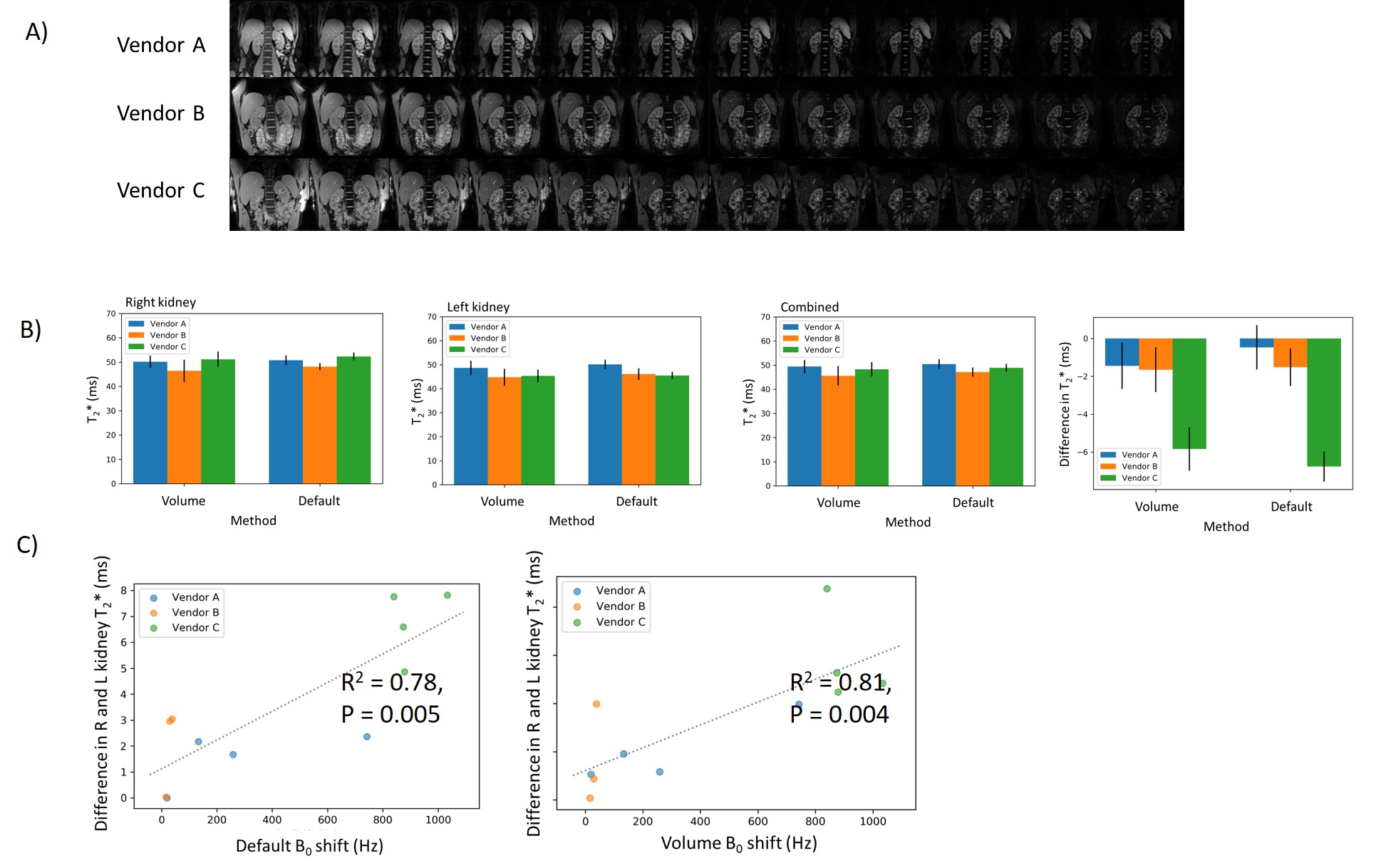
BOLD T₂* mapping: Multiple gradient echo sequence acquired using in-phase echoes (TE1/ΔTE = 4.21/4.21ms, 12 echoes, 5 slices, fat saturation, 3 breath holds). Datasets were collected for both ‘default’ and ‘volume’ shim settings.
B₁ field map: Acquired using the available B₁ mapping scheme for each vendor (DREAM/ TurboFLASH B₁ mapping /Bloch-Siegert method).
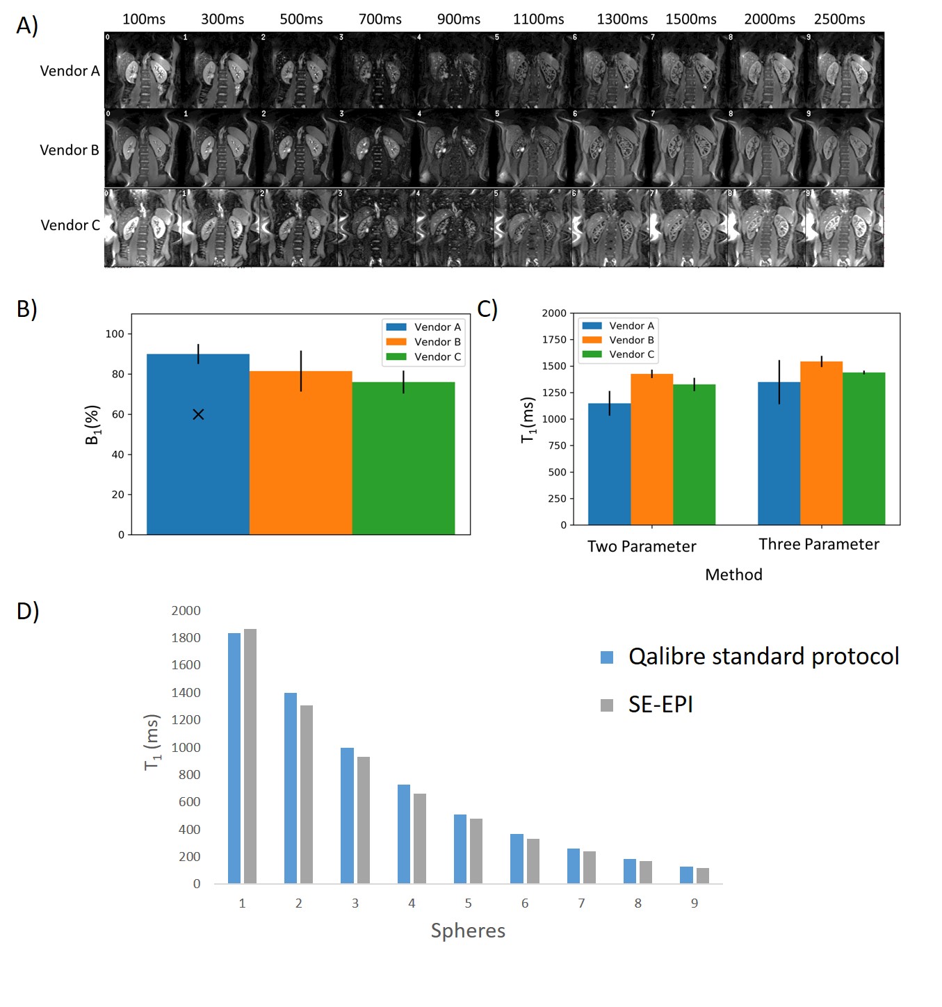
T₁ mapping: Spin-echo echo-planar-imaging (SE-EPI) inversion recovery (IR) data acquired (single slice, SENSE2, FA90,TR 6000ms,TE 27ms) respiratory triggered with data collected at 10 inversion times (100/300/500/700/900/1100/1300/1500/2000/2500ms).
Data Analysis: B₀ field maps were generated online (Philips, GE) or using FSL (Siemens). B₁ field maps were generated using online software. BOLD T₂* maps were fit to a log-linear decay function (for M₀, T₂*). Inversion recovery data was fit to a 2-parameter (for M₀ and T₁, assuming a perfect inversion) and 3-parameter fit (fitting for inversion efficiency, M₀ and T₁). Whole kidney ROIs were segmented manually from the magnitude data for both B₀ and B₁ maps, whilst cortex ROIs were generated for the T₁ and T₂* datasets. For each measure, the mode of the histogram of parameter values for each kidney was computed, from which the difference in measures between right and left kidney was calculated.

RESULTS

Figure 1 shows the L-R bias in B₀ across the abdomen for each shim setting and vendor. There was a significant difference in the B₀ L-R offset between vendors, with Vendor B consistently having the lowest offset and Vendor C the highest (Fig. 1B). There was a significant correlation of B₀ L-R offset for ‘default’ and ‘volume’ shim settings, and for 2D and 3D B₀ readout schemes (Fig. 1C). Figure 2 shows the BOLD T₂* data, a clear systematic difference in T₂* values is evident between left and right kidneys, with the greatest difference for Vendor C (Fig 2B). Figure 2C shows there was a significant correlation of the measured B₀ L-R offset with T₂* difference between left and right kidneys (default shim: R² = 0.78, p = 0.005, volume shim: R² = 0.81, p = 0.004), highlighting that the asymmetry in B₀ results in T₂* asymmetry. Figure 3A shows example T₁ mapping data across inversion times, whilst Figure 3B shows the variation in the mean B₁ (as percentage of requested flip angle) within the kidneys, this was not significantly different between vendors. T₁ values were found to be consistently lower for Vendor A and C than Vendor B for the 2-parameter fit, as expected the 3 parameter increases the T₁ values but discrepancy remains between vendors (Fig. 3C). Figure 3D shows the calibration of Vendor C against a standard of the Qalibre phantom.

DISCUSSION

Here we assess the intra-individual, inter-vendor comparisons of renal T₁ and BOLD T₂* measures using predominantly product sequences. We demonstrate that renal T₂* is sensitive to dephasing due to concomitant gradient magnetic fields, the degree of which is shown to vary across MR vendors. This B₀ L-R gradient leads to an asymmetry in T₂* values between L and R kidneys. Future work will address minimizing these B₀ variations. B₁ maps are shown to vary across subjects and vendors, but there was no vendor-specific bias. Renal cortex T₁ values computed using a simple 2-parameter fit (assuming 100% inversion efficiency) were shown to systematically vary across vendors, as expected a 3-parameter fit reduced this bias however differences remain. It should be noted that this difference in T₁ values may be due to the slice-selective inversion profile used by Vendors A and C, whilst Vendor B uses a non-selective inversion and is thus less prone to inflow effects, slice profile effects of the slice selective inversion and slice motion due to respiration.

CONCLUSION

To understand the difference in inter-vendor relaxometry measures, characterisation of the B₀ and B₁ field maps is essential. Underlying B₀ bias leads to alterations in renal T₂*, which should be accounted for in analysis, particularly for multi-centre studies. Further optimisation of T₁ measures are required to overcome systematic differences across vendors

Acknowledgements

This work is funded by MRC Partnership grant MR/R02264X/1.