INTRODUCTION

3D multi-echo gradient echo (GRE) acquisition in a breath-hold setting is typically used for water/fat separation to calculate of proton density fat fraction (PDFF), R2*, and field to be used for quantitative susceptibility mapping. The single breath-hold acquisition is tens of seconds to be manageable for patients in clinical practice (1,2). However. in elderly and paediatric patients long breath-holds might not be feasible. Compressed sensing along with Deep Learning is an alternative to shorten the scan time and perform reconstruction on undersampled data. In this work we compare how undersampling at different rates and use of Deep Learning for reconstruction will affect the water/fat separation output results.

METHODS

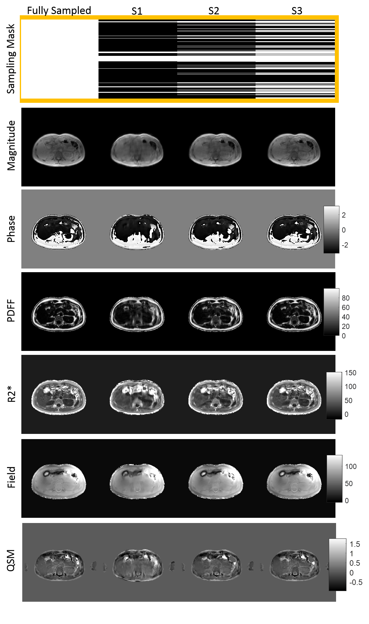
3D multi-echo gradient-echo breath-hold seqeunce was used to acquire complex data in both healthy volunteers (n=21) and patients (n=19) in 3 different scanners including two 1.5T GE scanners (Signa HDxt, GE Healthcare, Waukesha, WI) with 8-channel cardiac coils and a 1.5T Siemens scanner (Magnetom Aera, Siemens Healthcare, Erlangen, Germany) with 18-channel body coil. The GRE imaging parameters on the GE scanners: number of echoes = 6, unipolar readout gradients, flip angle = 5°, TE_1 = 1.2 msec, ∆TE = 2.3 msec, TR = 14.6 msec, acquired voxel size = 1.56×1.56×5 mm3, BW = 488 Hz/pixel, acquisition matrix = 150×150×(32-36) , ASSET acceleration factor = 1.25, and acquisition time of 20-27 sec. The GRE imaging parameters on the Siemens scanner: number of echoes = 6, unipolar readout gradients, flip angle = 5°, TE_1 = 1.7 msec, ∆TE = 2.3 msec, TR = 15 msec, acquired voxel size = 2.2×1.56×8 mm3, BW = 1500 Hz/pixel, acquisition matrix = 256×192×(28-36), slice and phase Fourier encoding = 7/8, GRAPPA acceleration factor = 2, and acquisition time of 22 sec.

Complex data were retrospectively undersampled with a random cartesian scheme at 3 different rates to achieve S1=14%, S2=28.9%, S3=50.7% density masks compared to fully sampled data. The Variational Network framework was used to perform reconstruction on these undersampled complex data (3):
$$u=argmin|{Au-f}|^2_2+\Sigma_{i=1}^{N_k}\phi_i(K_iu_i) [1]$$
where A denotes point-wise multiplication of Fourier operator and sampling mask to reconstruct images (u) from undersampled k-space data (f). The second term includes$$$N_k$$$ filters where the kernels ($$$K_i$$$) and non-linear potential functions ($$$Φ_i$$$) are learned during training (3). Complex data (256×256×1554×6) including magnitude/phase was split into 90% training and the rest for testing. The network included 10 layers, 30 filters with kernel size of 7×7, 5 batches, and learning rate of 1e-3.

Once GRE data from undersampled data were reconstructed, the T2*-IDEAL problem was solved to calculate fat content (F), water content (W), susceptibility induced field (f) and R2* decay from the reconstructed signal (u) shown in Eq.2:

$$(W,F,f,R_2^* )=argmin\sum_{j=1}^n|{u(t_{j})-e^{-R_2^*t_{j}}e^{-i2{\pi}ft_{j}}(W+F)e^{-i2{\pi}\nu_{f}t_{j}}}|^2_2 [2]$$
QSM was reconstructed using the MEDI algorithm (2),
$$\chi=argmin|{w(e^{-if}-e^{-i(d*\chi)})}|^2_2+{\lambda_1}|{M_{G}\triangledown\chi}|_1+{\lambda_2}|{M_{aorta}(\chi-\overline{\chi_{}}_{aorta})}|^2_2 [3]$$

w is the noise weighting (4), f the local field, d the dipole kernel, $$$M_G$$$ the binary edge mask, $$$\lambda_{1,2}$$$ regularization parameters, and $$$M_{aorta}$$$ the binary mask of abdominal aorta used for zero-referencing (5).
To compare fully sampled data with the reconstructed GRE data at different sampling rates, peak signal-to-noise ratio (PSNR) and structural Similarity Index (SSIM) are reported. To compare water/fat separation and QSM results from fully sampled data with the undersampled results, ROIs were drawn on PDFF (|F|/(|W|+|F|)), R2*, field and QSM maps in the liver and subcutaneous fat and relative error is reported.

Results

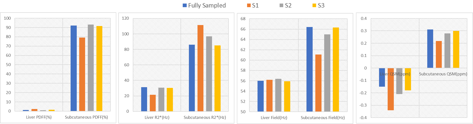
In Figure 1, 1st echo magnitude and phase along with water/fat separation outputs (PDFF (%), R2*(Hz), and field (Hz)) and QSM maps are shown. There is low qualitative agreement between the ground truth and reconstructed undersampled data with 14% density mask (S1) and improves at higher density (S2, S3). In Table.1, PSNR (dB) increases from 27.3 to 37.6 dB as sampling density increases and SSIM increases from 0.94 to 0.98

In Figure 2, PDFF ROI analysis shows that S1 has the highest relative errors (liver -50%, subcutaneous 16.3%). S2 has lower relative errors (liver 33%, subcutaneous -1.2%) and the best agreement with the lowest error is S3 (liver -25%, subcutaneous 0.4%). Note that errors in liver are higher due to minimal fat in healthy volunteers. R2* ROI analysis shows that S1 has the highest relative error (liver 46%, subcutaneous -22%). S2 has lower relative error (liver 1.9%, subcutaneous -11%) and the best agreement with the lowest error in S3 (liver 3.6%, subcutaneous 1%). Field ROI analysis shows that S1 has good agreement (liver -0.3%, subcutaneous 8.6%) and the results improve in S2 (liver -0.7%, subcutaneous 2.1%) and S3 (liver 0.1%, subcutaneous 0.1%) suggesting phase date is less susceptible to undersampling artifacts. QSM ROI analysis shows that S1 has low agreement with relative error (liver -55%, subcutaneous 42.8%) and results improve in S2 (liver -28%, subcutaneous 10.7%) and S3 (liver -16%, subcutaneous 3.6%).

CONCLUSION

This work shows feasibility of compressed sensing along with Deep-Learning reconstruction to shorten the scan time using 3D GRE sequence for the purpose of water/fat separation and QSM generation. While the undersampling with up to ~30% density mask provides reliable maps for quantitative analysis lower sampling masks suffer significantly from artifacts.

Acknowledgements

No acknowledgement found.