Introduction

Prostate cancer (PCa) is one of most common malignant tumors in man [1]. The accurate detection of PCa is a challenging task in clinic [2]. The distinction of PCa from benign conditions, including benign prostatic hyperplasia (BPH) and prostatitis, is critical to personalized medicine [3]. Currently, MR images of the prostate are evaluated by radiologists. However, the detection and diagnosis of PCa using MR images varies considerably [4]. Quantitative imaging features may provide additional information for differentiation of the benign and malignant lesions. Furthermore, deep learning using convolutional neural network provides a fully automatic and efficient approach to analyze detailed information in the tumor and the surrounding per-tumor tissue for diagnosis. The goal of this study is to evaluate the accuracy of prediction using the SVM model based on the histogram and texture features extracted from the lesion, as well as deep learning using three different networks. The results to differentiate between prostate cancer and benign prostatic hyperplasia are compared.

Methods

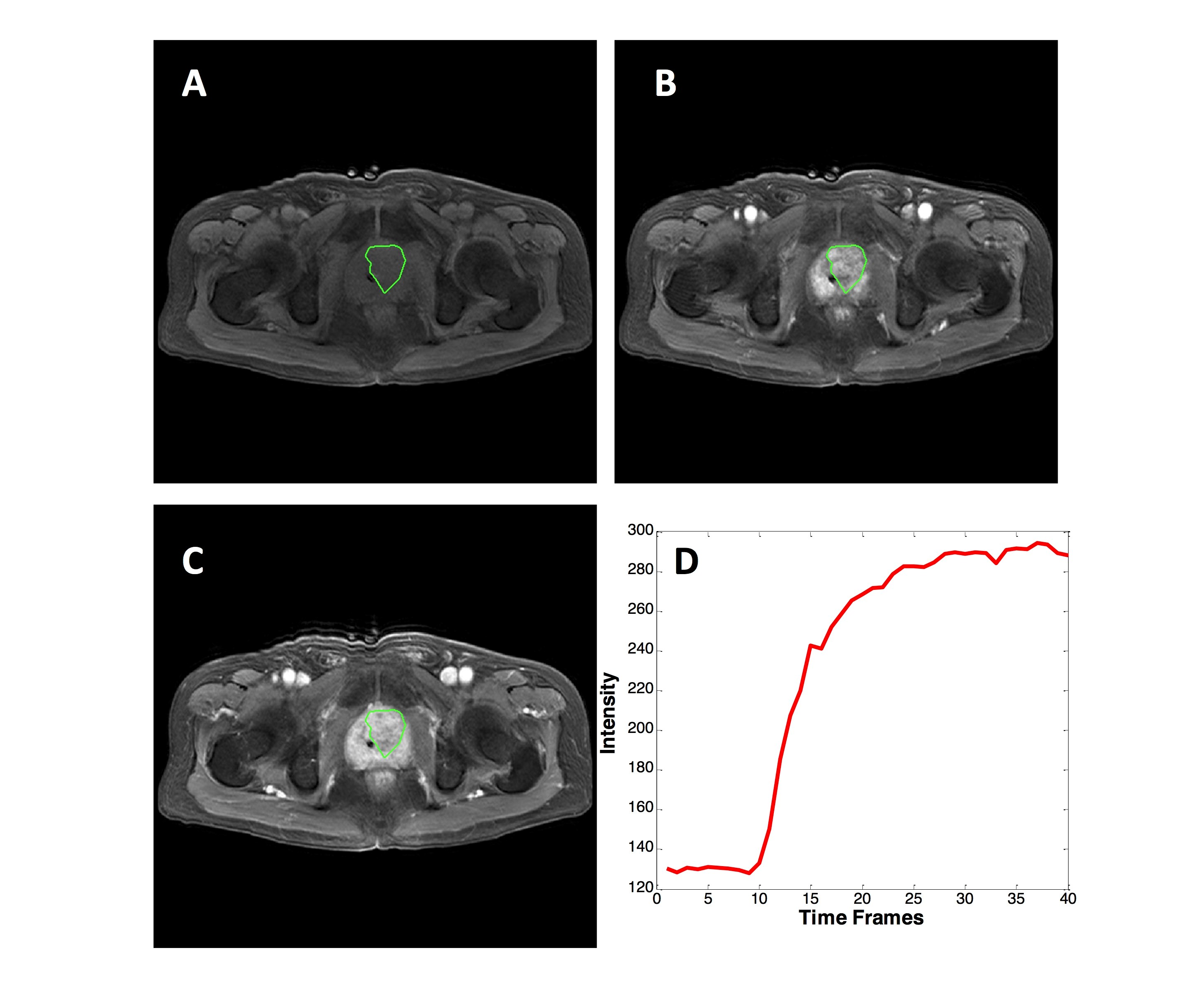
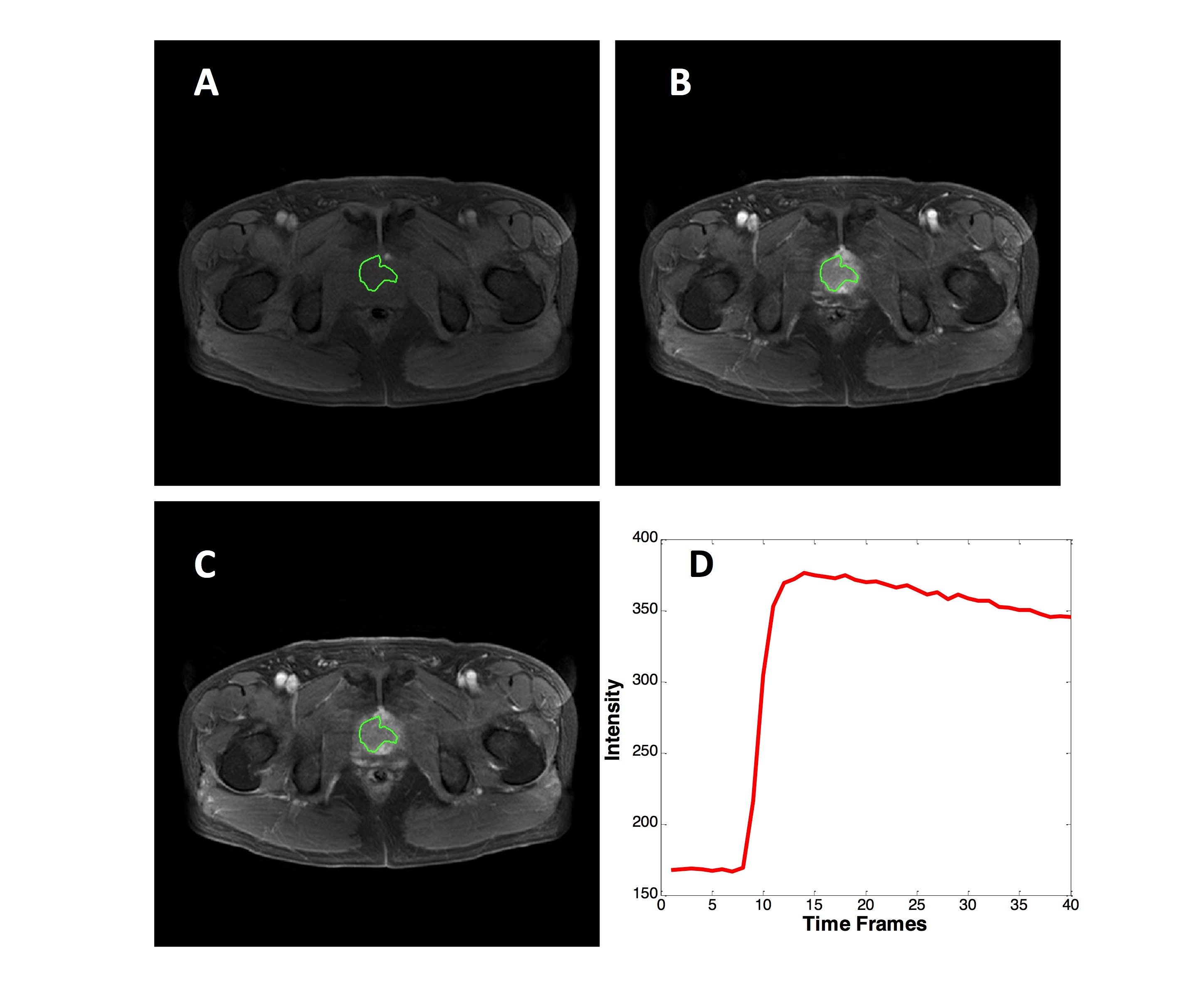
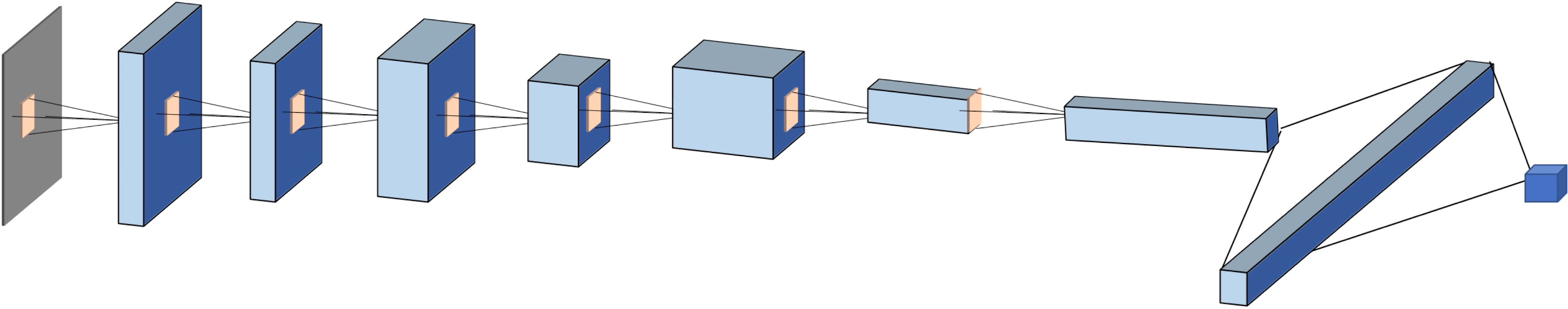
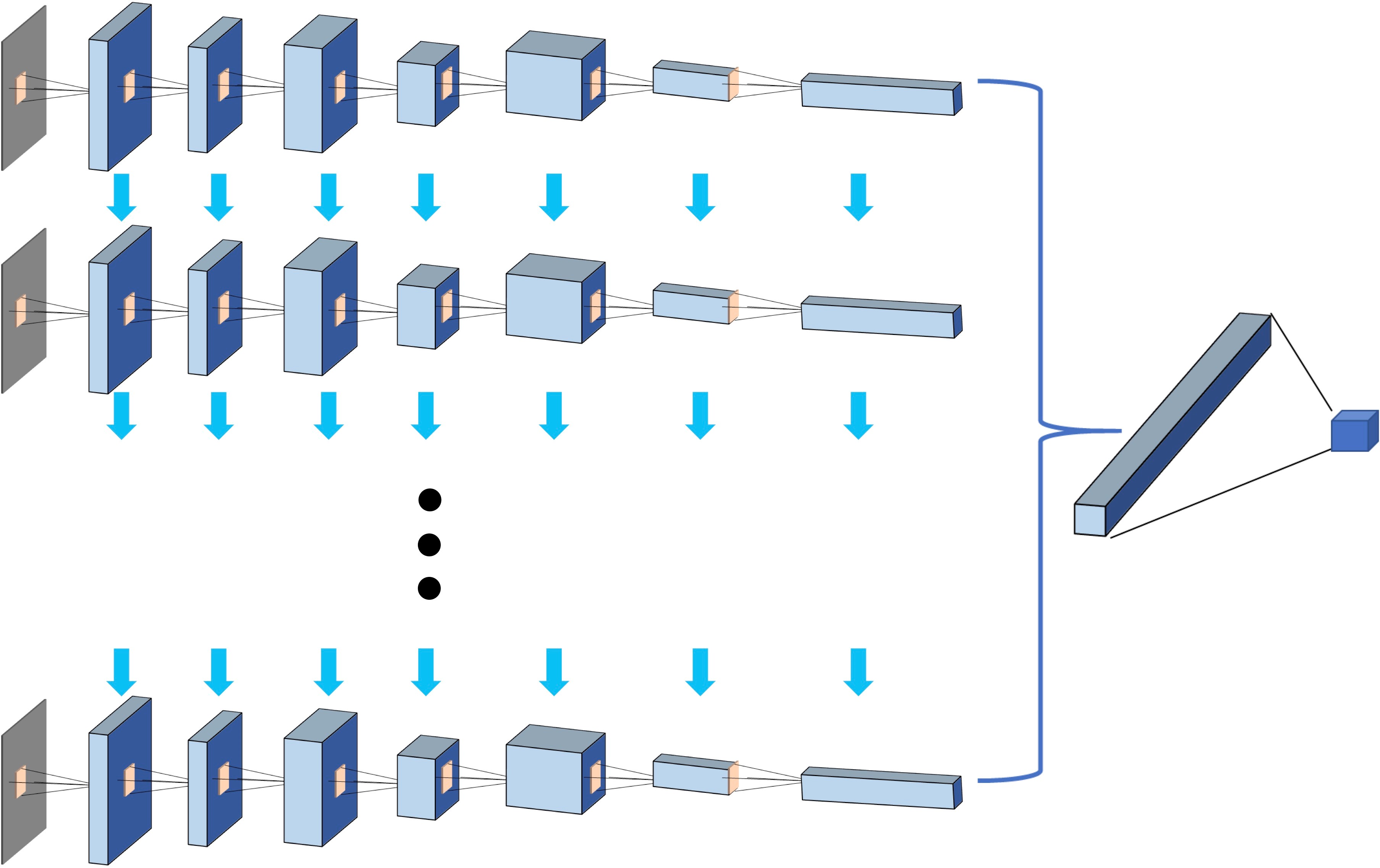
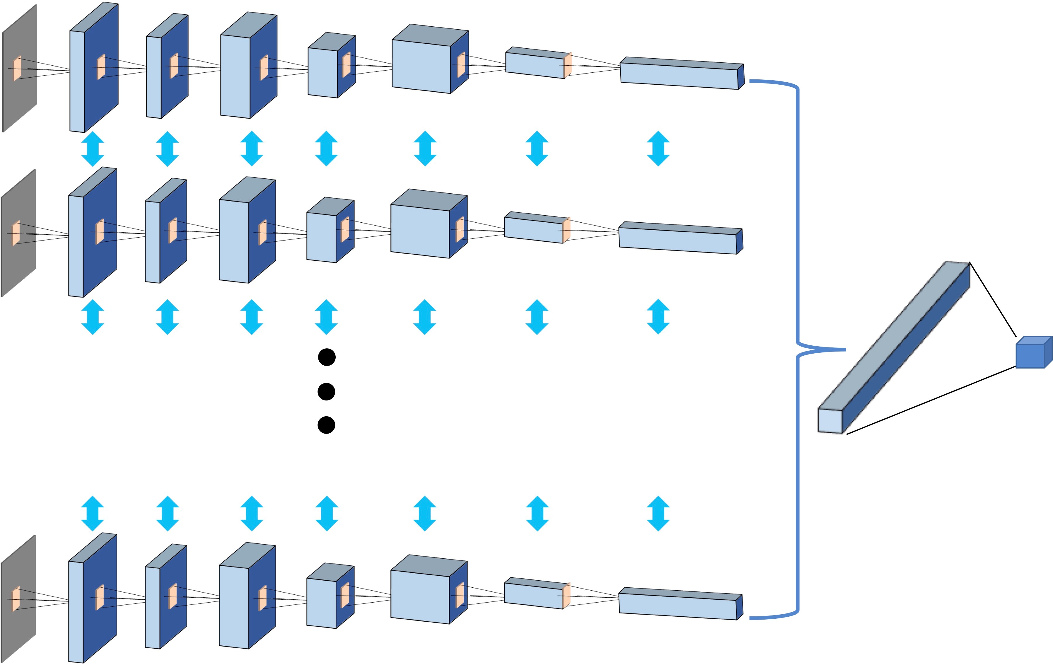
From September 2014 to September 2018, 67 patients underwent prostate multi-parametric MRI (mpMRI) and were confirmed with PCa by transrectal ultrasonography guided prostate biopsy and followed radical prostatectomy. 37 BPH patients underwent mpMRI showing PI-RADS v2≤2, and they received biopsy in an interval less than 6 months and were confirmed to have negative findings. MR examinations were carried out on a 3.0 T scanner (Achieve; Philips, The Netherlands) equipped with a sixteen-channel sensitivity-encoding (SENSE) torsor coil without an endorectal coil. Four hours of fasting prior to MR examination was required to suppress bowel peristalsis. During the acquisition, a contrast agent (Omniscan, GE, concentration: 0.5 mmol/ml) with a dose of 0.2 ml/kg of body weight at a flow rate of 2 ml/s was injected via a power injector (Spectris Solaris EP, Samedco Pvt Ltd) at the start of the sixth DCE time point followed by a 20 ml saline flush. Figures 1 and 2 show two case examples. Only the DCE images were analyzed in this study. A total of 40 frames were acquired, including 5 pre-contrast (F1-F5) and 35 post-contrast (F6-F40). Two radiologists outlined the whole prostate gland and the index suspicious lesion in consensus on DCE-MRI using imageJ (NIH, USA). The outlined lesion ROI on all slices were combined to generate a 3D tumor mask, and 13 histogram features and 20 GLCM texture features were extracted on each DCE images, with a total of 33x40=1320 features. For differentiation between BPH and PCa using a radiomics method, feature selection was first implemented by using an SVM based sequential feature selection methods to find features with the highest significance. These features were then used to train a final SVM model with Gaussian kernel to serve as the diagnostic classifier. For deep learning, first, a VGG network with 8 convolutional layers were implemented to differentiate between BPH and PCa patients. The 5 pre-contrast frames were averaged as the reference for normalizing post-contrast frames. The last 20 frames were down-sampled to 10 frames, by only selecting every other frame. So, a total of 25 normalized enhancement maps were used. Figure 3 shows a VGG network architecture which used all 25 sets of images as input without timing information. Then, to consider the change of the signal intensity with time, a convolutional long short term memory (CLSTM) network was applied, shown in Figure 4. The 25 sets of enhancement maps were added one by one into the network. However, due to the forgot gate implemented in LSTM, information from early time points contributes less than later time points. To minimize this problem, a bi-directional CLSTM model was applied, shown in Figure 5. To investigate the contribution from the peri-tumor tissue, region growing was utilized to include connected pixels with the outlined tumor ROI, where the enhancement was > 10% of the mean tumor ROI enhancement on the 10th DCE frame. The results obtained using the expanded ROI and the tumor ROI were compared. To avoid overfitting, the dataset was augmented by random affine transformation. The algorithm was implemented with a cross entropy loss function and Adam optimizer with initial learning rate of 0.001.

Results

The accuracy for differentiating between BPH and PCa was 0.81 when using the SVM model built based on the histogram and texture parameters. In deep learning using VGG with the manually outlined ROI as inputs, the accuracy in 10-fold cross-validation was 0.64 – 0.77 (mean: 0.68). When considering the DCE time frames, the accuracy was improved to 0.75 – 0.87 (mean: 0.81) using one-directional CLSTM architecture, and further to 0.73 – 0.89 (mean: 0.84) using the bi-directional CLSTM architecture. When considering the peri-tumor tissues using expanded ROI as inputs, the accuracy of the bi-directional CLSTM was decreased to 0.68-0.85 (mean: 0.78), which was worse compared to the results obtained using the manually drawn ROI as inputs.

Discussion

In this study we elucidated that prostate DCE-MR images can be analyzed using SVM and deep learning classifiers to differentiate between PCa and BPH patients. The recurrent network using CLSTM could take the change of signal intensity in the DCE series into consideration, and the accuracy was higher compared to the conventional VGG. The train of 40 DCE frames might be too long for CLSTM, so they were down-sampled to 25 by skipping every other frame in the last 20 frames. To further investigate whether the early information, which usually captured the important wash-in phase, was lost in one-directional CLSTM, the bi-directional CLSTM was implemented, and the mean accuracy was improved to 0.84. The results suggest that although the CLSTM is an efficient approach for considering images acquired in a time series, the train length needs to be considered, and novel approaches such as the bi-directional analysis can be considered. When the peritumoral information outside the lesion ROIs was considered, the prediction accuracy was worse, which could be due to the diluted information by including the weakly enhanced tissues into analysis. This study demonstrates that machine learning using radiomics and deep learning, with appropriate consideration of the time series, can be implemented to analyze the DCE-MRI to differentiate between PCa and BPH.

Acknowledgements

This study was supported by NIH CA127927.