2317
Implementing compressed sensing with deep image prior to reconstruct undersampled dynamic contrast-enhanced MRI data of the breast1Physics, University of Texas at Austin, Austin, TX, United States, 2Oden Institute for Computational Engineering and Sciences, University of Texas at Austin, Austin, TX, United States, 3Livestrong Cancer Institutes, University of Texas at Austin, Austin, TX, United States, 4Electrical and Computer Engineering, University of Texas at Austin, Austin, TX, United States, 5Biomedical Engineering, University of Texas at Austin, Austin, TX, United States, 6Medicine, University of Texas at Austin, Austin, TX, United States, 7Biomedical Engineering, University of Alabama at Birmingham, Birmingham, AL, United States, 8Wireless Networking and Communications Group, University of Texas at Austin, Austin, TX, United States, 9Oncology, University of Texas at Austin, Austin, TX, United States
Synopsis
We evaluate the ability of the compressed sensing with deep image prior (CS-DIP) algorithm to reconstruct undersampled dynamic contrast-enhanced MRI data of the breast. The performance of the reconstruction is evaluated by comparing quantitative parameters computed from the reconstructed data to the original parameter values computed from fully-sampled data. We hypothesize that CS-DIP will enable dramatically fewer k-space measurements, thereby allowing for higher temporal (while maintaining spatial) resolution of breast MRI scans.
Introduction
Dynamic contrast-enhanced (DCE) MRI involves the serial acquisition of heavily T1-weighted MRI data which can then be analyzed with a pharmacokinetic model to return estimates of the volume transfer constant (Ktrans) and extravascular/extracellular volume fraction (ve) [1]. Ktrans has been shown to be an important diagnostic parameter, along with the semi-quantitative signal enhancement ratio (SER), as it differs significantly between malignant and benign tissues [2]; however, the ability to accurately and precisely determine these model parameters is fundamentally limited by the temporal resolution of the DCE-MRI protocol [3]. The potential to expedite temporal sampling without substantial reduction in spatial resolution has not been explored using compressed sensing with deep image prior (CS-DIP), which requires a very small data set for training [4]. Here we quantitatively compare the pharmacokinetic and semiquantitative analyses of fully sampled DCE-MRI data to that performed on DCE-MRI data that was retrospectively undersampled and reconstructed with CS-DIP.Methods
DCE-MRI acquisition. Patients (N=22) with locally advanced breast cancer were scanned using a 3T Skyra (Siemens, Erlangan, Germany) equipped with a 16-channel receive double-breast coil (Invivo, Gainsville, FL). DCE-MRI data was collected with an acquisition matrix of 192×192 and TR/TE/a = 7.02 ms/4.60 ms/6o and a GRAPPA acceleration factor of 2 so that each 10-slice set was collected in 7.3 s at 66 time points. After collecting one minute of dynamic scans (i.e., the first 8 time points), 10 mL of Gadavist (Bayer, Whippany, NJ) was delivered at 2 mL/sec (followed by a saline flush) through a catheter placed within an antecubital vein. One representative patient dataset was used for the preliminary analysis presented in this abstract.CS-DIP reconstruction. Each image frame of the representative DCE-MRI data set was first retrospectively under-sampled by applying a Cartesian binary sampling mask of 50 equidistant lines distributed along the phase encoding direction, corresponding to an improvement in temporal resolution of nearly a factor of four. The resultant k-space measurements were passed to the CS-DIP algorithm, implemented in Python, which trains the weights of a deep convolutional generative adversarial network (DCGAN) by minimizing the error between the measurements and the measured network output as well as the total variation of the output [4].
DCE-MRI analysis. The reconstructed DCE-MRI data were first segmented using the Fuzzy C-means algorithm [5]. The dynamic times courses from the tumor region of interest (ROI) were then analyzed by the Kety-Tofts model implemented in MATLAB (Mathworks, Natick, MA) to return Ktrans and ve parameter maps. Fits were bounded such that Ktrans is constrained between 0 to 5 min-1 and ve is constrained between 0 to 1. Semiquantitative SER maps were also computed using the reconstructed data. Note, these parameter maps are subsequently referred to as “reconstruction-based”. The same procedure was applied to the original DCE-MRI time courses to obtain ground truth parameter estimates and SER maps (subsequently referred to as “original”) to which the reconstruction-based parameter estimates and SER values were compared.
Statistical analysis. The percent error and concordance correlation coefficient (CCC) between the original and reconstructed parameter estimates were evaluated to determine the accuracy of using a pharmacokinetic analysis of CS-DIP reconstructed DCE-MRI data. The percent error, CCC, and structural similarity index (SSIM) were employed to evaluate the quality of the reconstructed image frames compared to the original dataset. The CCC and SSIM extend from -1 (complete disagreement) to 1 (complete agreement).
Results
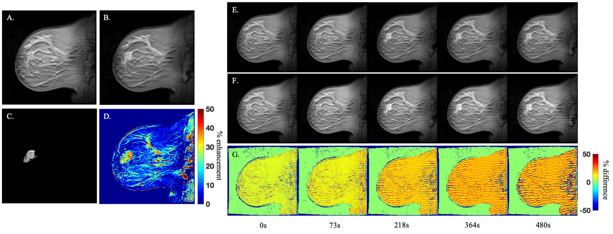
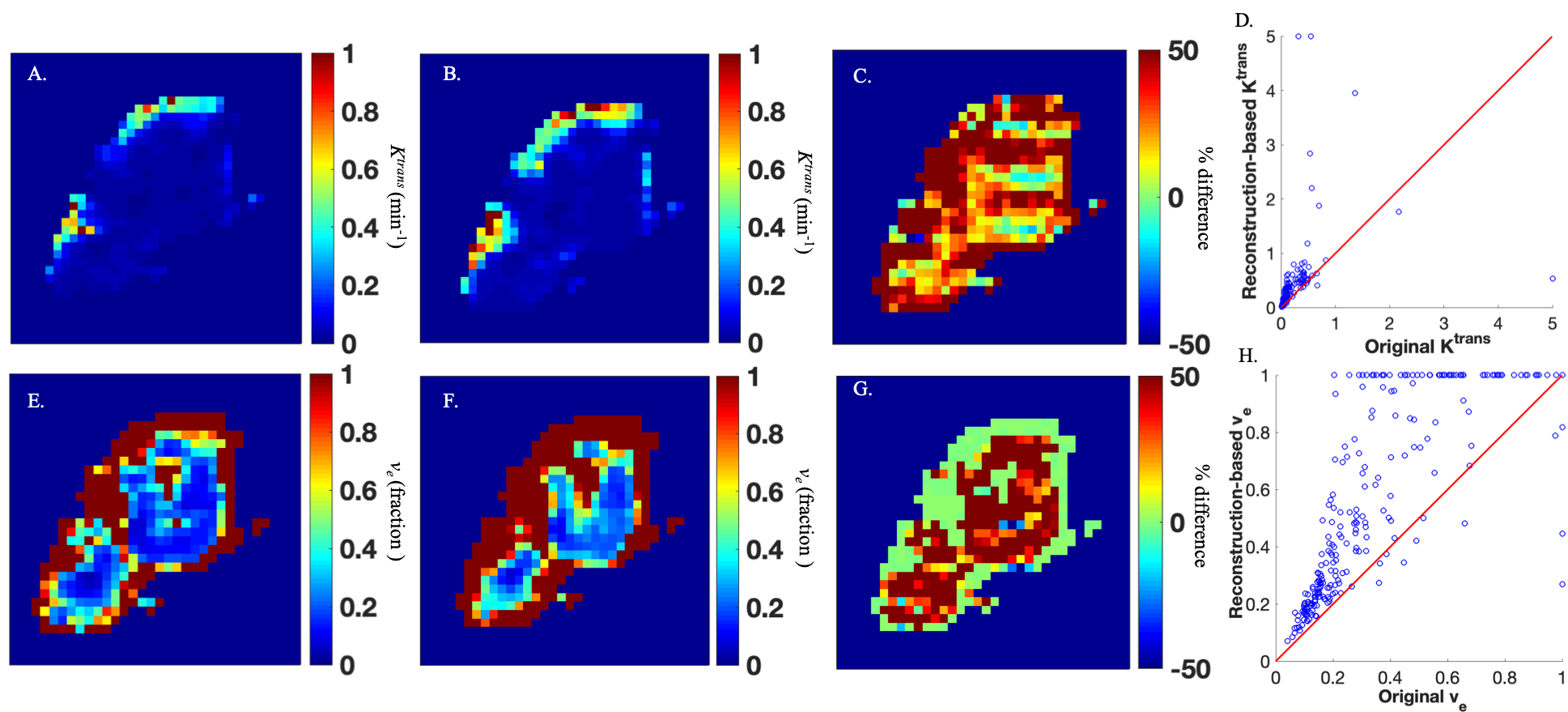
The comparison of example time points 1 , 10, 30, 50, and 66 from the reconstructed and original DCE-MRI time courses are presented in Figure 1 as a set of percent difference maps. The average percent error, CCC, and SSIM over the breast tissue across all 66 frames are approximately 17%, 0.73, and 0.56, respectively.The comparison of the reconstruction-based and original parameter maps are presented in Figure 2 as a set of percent difference maps alongside the parameter maps themselves. The average percent error and CCC across the tumor ROI for Ktrans was 71% and 0.37, respectively, while for ve it was 47% and 0.80, respectively.
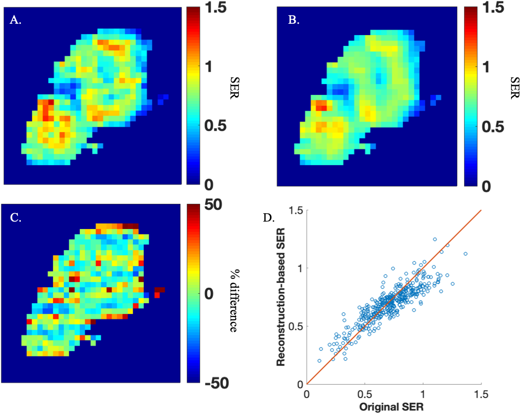
Finally, the comparison of the reconstruction-based and original SER maps are presented in Figure 3. The average percent error and CCC for SER across the tumor ROI was 13% and 0.85, respectively.
Discussion and Conclusion
In this preliminary work, we have achieved the first application of CS-DIP to DCE-MRI data. While pure compressed sensing (CS) reconstruction has yielded higher agreement in Ktrans, ve, and SER from DCE-MRI breast data (i.e,, average percent difference of 12% in Ktrans parameter maps for 4x compression) [6], CS-DIP has been shown to outperform CS in radiography, retinopathy, and MNIST images [4]. It is reasonable to hypothesize similar results from our current framework by refining the DCGAN architecture in a manner that optimizes the reconstruction of DCE-MRI data. Additionally, deep neural networks are notorious for requiring large training data sets, but CS-DIP necessitates as few as a single training image [4]. This is an attractive feature as DCE-MRI frames are highly correlated outside of the enhancing region. We continue to test this promising method by refining the DCGAN architecture and building a pipeline to reconstruct all N=22 patients currently in our dataset at multiple compression factors.Acknowledgements
We thank the the National Cancer Institute for funding through NCI U01CA142565 and U01CA174706 and also the Cancer Prevention and Research Institute of Texas for funding through CPRIT RR160005. This work has also been supported by NSF Grants 1618689, DMS 1723052, CCF 1763702, AF 1901292 and research gifts by Google, Western Digital.References
[1] Yankeelov TE & Gore JC. Dynamic Contrast Enhanced Magnetic Resonance Imaging in Oncology: Theory, Data Acquisition, Analysis, and Examples. Curr Med Imaging Review. 2009;3(2): 91-107.
[2] Sorace AG, Partridge SC, Li X, Virostko J, Barnes SL, Hippe DS, Huang W, & Yankeelov TE. Distinguishing benign and malignant breast tumors: preliminary comparison of kinetic modeling approaches using multi-institutional dynamic contrast-enhanced MRI data from the International Breast MR Consortium 6883 trial. Journal of Medical Imaging. 2018;5(1):011019.
[3] Levine E, Daniel B, et al. 3D Cartesian MRI with Compressed Sensing and Variable View Sharing Using Complementary Poisson-disc Sampling. Magn Reson Med. 2017; 77(5):1774-1785.
[4] Van Veen D, Jalal A, Soltanolkotabi M, Price E, Vishwanath S, & Dimakis AG. Compressed Sensing with Deep Image Prior and Learned Regularization. arXiv preprint. 2018; arXiv:1806.06438.
[5] Chen W, Giger ML, Bick U. A fuzzy C‐means (FCM)‐based approach for computerized segmentation of breast lesions in dynamic contrast‐enhanced MR images. Acad Radiol. 2006;13:63–72.
[6] Smith DS, Welch EB, Li X, Arlinghaus LR, Loveless ME, Koyama T, Gore JC, & Yankeelov TE. Quantitative Effects of Using Compressed Sensing in Dynamic Contrast Enhanced MRI. Phys. Med. Biol. 2011; 56: 4933-4956
Figures