2279
A Direct Variational Pressure Estimation Approach for Velocity Data in 4D Flow MRI
Lixing Ren1,2, Xiaowei He2, Dandan Zheng3, and Enhua Wu2,4
1University of Chinese Academy of Sciences, Beijing, China, 2The State Key Lab. of CS, Institute of Software, Chinese Academy of Sciences, Beijing, China, 3Clinical Science, Philips Healthcare, Beijing, China, 4University of Macau, Macau, China
1University of Chinese Academy of Sciences, Beijing, China, 2The State Key Lab. of CS, Institute of Software, Chinese Academy of Sciences, Beijing, China, 3Clinical Science, Philips Healthcare, Beijing, China, 4University of Macau, Macau, China
Synopsis
Understanding the nature of the pressure changes is crucial for diagnosis and therapy strategy optimization for aortic aneurysm. 4D flow MRI had offered the opportunity to assess 3D blood flow characteristics. However, the pressure quantification is still a challenge due to the low signal-to-noise ratio and the partial volume effects near the wall. The focus of this work is to address this deficiency by proposing a novel workflow of direct pressure estimation based on simulated noisy 4D flow MRI data.
Introduction
In aortic aneurysm, which is a common cause of morbidity and mortality1, the spatial distribution and temporal changes of pressure in aortic are critical in initiating complications such as dissection and rupture. Understanding the nature of these pressure changes is crucial for diagnosis and therapy strategy optimization. 4D flow MRI had offered the opportunity to assess 3D blood flow characteristics. However, the pressure quantification is still a challenge because of the low signal-to-noise ratio and the partial volume effects near the wall2. The focus of this work is to address this deficiency by proposing a novel workflow to study direct pressure estimation based on simulated noisy 4D Flow MRI data.Methods
To evaluate the accuracy of pressure estimation for 4D Flow MRI data tainted by noise, blood is modeled as an incompressible inviscid fluid governed by the following Navier-Stokes equations$$\frac{\partial \mathbf{u}}{\partial t}=-\mathbf{u}\cdot \triangledown \mathbf{u}-\frac{1}{\rho}\triangledown p, subject\;to\;\triangledown \cdot \mathbf{u}=0$$where $$$\mathbf{u}$$$ is blood velocity, $$$p$$$ is blood pressure and blood density $$$\rho$$$ is set to $$$1060kg/m^{3}$$$. Figure 1 demonstrates an overview of our estimation-simulation scheme.Synthetic data. A segmented aortic arch is selected as the vessel wall for blood simulation. Velocity profiles extracted from the in vivo measurements and zero pressure were used as inlet and outlet boundary conditions (BCs), respectively. A standard finite volume method (FVM) was used to generate velocity and pressure sequences over one cardiac cycle. To mimic the acquisition of 4D Flow MRI data, both the 3D velocity and pressure fields were extracted from the sequence every 40ms. During the extraction, white noises with different intensities were added to mimic experimental data with uncertainty.
Pressure computation. To estimate the pressure field based on two successive velocity fields, a variational energy formulation is proposed as follows $$E^{n+1}=(\mathbf{u}_s^{n}-\frac{\delta t}{\rho}\triangledown p)^{T} \mathbf{W}(\mathbf{u}_s^{n}-\frac{\delta t}{\rho}\triangledown p)+\lambda (\mathbf{u}_s^{n}-\frac{\delta t}{\rho}\triangledown p-\mathbf{u}_s^{n+1})^{T}\mathbf{W}(\mathbf{u}_s^{n}-\frac{\delta t}{\rho}\triangledown p-\mathbf{u}_s^{n+1})$$where $$$\mathbf{u}_s^{n}$$$ and $$$\mathbf{u}_s^{n+1}$$$ denote the extracted velocity field at time n and n+1, $$$\delta t$$$ denotes the time interval (which is 40ms in our current setting), $$$\mathbf{W}$$$ is a diagonal matrix with each entry representing the fraction of blood occupying each voxel. Minimizing the first term of $$$E^{n+1}$$$ with respect to pressure $$$p$$$ is equivalent to enforcing $$$\mathbf{u}_s^{n}$$$ to be divergence-free3. Minimizing the second term of $$$E^{n+1}$$$ guarantees the final velocity should not deviate too far from the exacted velocity $$$\mathbf{u}_s^{n+1}$$$. $$$\lambda$$$ is a positive control parameter to balance the effects of above two terms.
Results
Figure 2 shows a comparison of pressure estimation error compared to the CFD-generated pressure field, where 10% white noise were added to CFD-generated velocity fields during the velocity extraction. To compare the effectiveness of our direct pressure estimation method, an alternative solution involving divergence-free smoothing (DFS)4 for $$$\mathbf{u}_s^{n}$$$ and $$$\mathbf{u}_s^{n+1}$$$ is also implemented, it can be noted that the pressure field is sensitive to velocity smoothing. Instead, our direct variational pressure estimation method is able to decrease the pressure estimation error up to 95%. Additionally, the pressure estimation accuracy with different intensities of white noise were examined in Figure 3, corresponding to white noise intensities of: 0%(i.e., no noise), 5%, 10%, 15% and 20%.Discussion
Computational results for pressure show that the accuracy of pressure estimation could be largely affected by noise. Velocity smoothing helps to reduce the divergence error in velocity fields, nevertheless, it does not help improve the accuracy in computing the pressure field according to our experiments. Our direct variational pressure computing method shows improved accuracy in resisting noise during acquisition. Concerning limitations, this study did not asses the accuracy of our method on actual 4D Flow MRI imaging data yet. Further evaluation is required to confirm the accuracy compared to other boundary conditions5, numerical solvers6 as well as pressure measured by intravascular catheterization.Conclusion
A direct variational approach applicable to wall-bounded flow has been developed for computing pressure field from velocity data generated from CFD simulation. The results indicate that it has a good anti-noise capability. It is expected to improve the estimation accuracy of pressure required for the reliable diagnosis of cardiovascular diseases with 4D flow MRI.Acknowledgements
This work was supported by the the National Key R&D Program of China (No. 2017YFB1002700), the National Natural Science Foundation of China (No.6187070657) and Youth Innovation Promotion Association, CAS (No.2019109).References
- Anjum A, Von Allmen R, Greenhalgh R, Powell JT. Explaining the decrease in mortality from abdominal aortic aneurysm rupture. Br J Surg. 2012;99:637–645.
- Pablo Lamata, Alex Pitcher, Sebastian Krittian, et al. Aortic Relative Pressure Components Derived from Four-Dimensional Flow Cardiovascular Magnetic Resonance. Magnetic Resonance in Medicine.2014: 72:1162–1169
- Christopher Batty, Florence Bertails, and Robert Bridson. A fast variational framework for accurate solid-fluid coupling. ACM Trans. Graph. 2007, 26, 3, Article 100. DOI: https://doi.org/10.1145/1276377.1276502
- Wang C, Gao Q, Wang H, Wei R, Li T, Wang J. Divergence-free smoothing for volumetric PIV data. Experiments in Fluids (2016) 57: 15. https://doi.org/10.1007/s00348-015-2097-1.
- Pirola S, Cheng Z, Jarral OA, O'Regan DP, Pepper JR, Athanasiou T, Xu XY. On the choice of outlet boundary conditions for patient-specific analysis of aortic flow using computational fluid dynamics. J Biomech. 2017 Jul 26;60:15-21. doi: 10.1016/j.jbiomech.2017.06.005. Epub 2017 Jun 20.
- Marlevi, D., Ruijsink, B., Balmus, M. et al. Estimation of Cardiovascular Relative Pressure Using Virtual Work-Energy. Sci Rep 9, 1375 (2019) doi:10.1038/s41598-018-37714-0
Figures
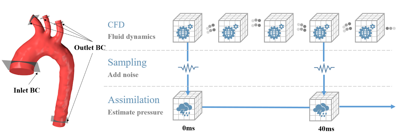
Figure 1: Overview of the estimation-simulation workflow.
Top: A standard finite volume method (FVM) was used to generate velocity and
pressure sequences over one cardiac cycle; Middle: Noise was added to the
velocity fields to mimic experimental data with uncertainty. Bottom: A direct
variational method to estimate pressure from two successive velocity fields.
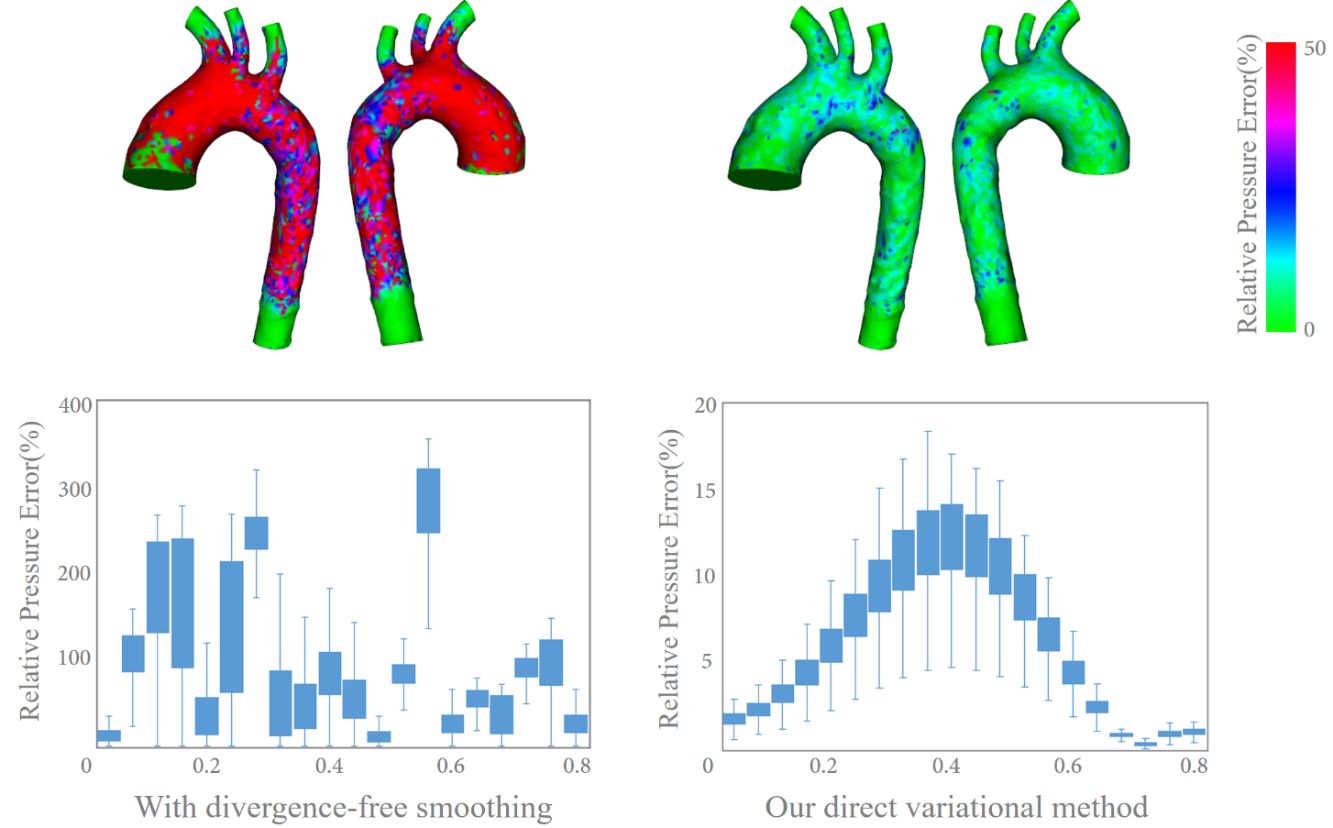
Figure 2: A comparison the effectiveness of our direct
pressure estimation method. Top: A comparison of the relative pressure error
distribution at t=0.36s; Bottom left: Time history of relative pressure error
when divergence-free smoothing is taken before pressure estimation; Bottom right:
Time history of relative pressure error with our direct variational method.
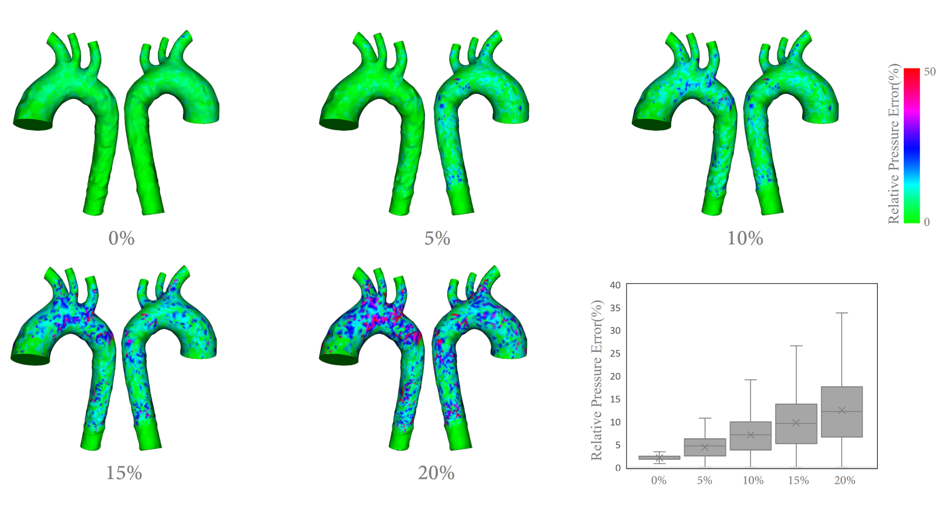
Figure 3: A comparison of the pressure estimation
accuracy with different intensities of white noise at t=0.36s.