2274
Combining variational methods and particle tracking in 4D Flow MRI for displacement artifact compensation1Institute for Biomedical Engineering, ETH Zurich, Zurich, Switzerland
Synopsis
We propose a variational method for reconstructing divergence-free velocity fields from 4D Flow MRI data with compensation of spatial displacement artifacts. A standard 4D Flow MRI sequence to measure flow velocities in an expanding flow phantom with Reynolds number of 4000 was used. A variational formulation allows to reconstruct a divergence-free velocity field used to estimate the displacement artefact associated with spin motion between the time point of motion encoding and echo time. The field was used to apply a spatial shift of the original MRI data and compute new divergence-free flow velocities corrected for spatial motion artifacts.
Introduction
The accuracy and precision of phase contrast (PC) 4D Flow MRI is compromised by noise, partial voluming, eddy current effects and other inconsistencies of encoding and decoding of velocity information1. One metric to assess the level of corruption of the measurements is the divergence of the reconstructed velocity vector fields1-2. Assuming blood to be incompressible, any variation from the zero-divergence condition can be attributed to errors in the measurements. Several methods have been proposed to correct and denoise flow measurements imposing fluid-dynamically consistent constraints2-3. They often require ad-hoc parameters calibration, particularly when they include penalization terms connected to the fluid momentum conservation. There is, however, a lack of an established consensus on the way to assess the improvement of the correction in in-vivo cases. An additional source of error is due to spatial or oblique displacement artifacts4 which are caused by the velocity-proportional displacement of magnetization during the time between motion (bipolar gradient) and spatial encoding (readout). In our approach, we aim at a velocity field which minimizes the difference with the original velocity with the sole constraint to be divergence-free. Moreover, displacement artefact are corrected by backwards-tracking of seeds placed in the nodes of a computational mesh and using the divergence-free velocity. The resulting spatial displacement is used to add a spatial shift to the MRI velocity fields which are then used for the calculation of a divergence-free velocity map corrected for spatial displacement artifacts.Methods
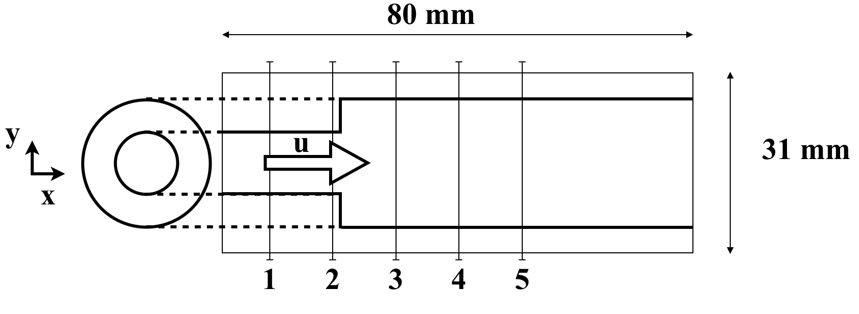
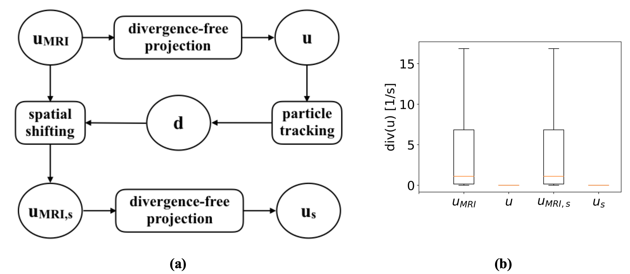
A standard 4D Flow MRI sequence was used on a 3T MR system to measure the velocity in an expanding steady flow phantom with diameter ratio of 2:1 (Figure 1), Reynolds number of 4000 (with reference to the larger diameter of 2 cm) and vmax = 158 cm/s. The spatial resolution was 2.5 mm isotropic and images were zero-filled to an isotropic resolution of 1.5 mm. A region-of-interest (ROI) around the main axis with length of 80 mm in the axial direction and 31 mm in the orthogonal directions was selected. Thereafter, a regular cubic grid with spatial resolution matching that of the data was generated, and subsequently transformed into tetrahedral elements preserving the nodes. PC-MRI velocities, uMRI, were thresholded to 0.4 of the maximum magnitude value in the ROI and then projected onto the mesh, while the remaining voxel values were set to zero. An initial divergence-free velocity field, u, was obtained by minimizing the difference between the reconstructed and original velocities, u and uMRI, respectively, subjected to a divergence-free constraint imposed as a Lagrangian multiplier5. This leads to a saddle-point problem that was solved in FEniCs6-9 using a FE mixed formulation5. Subsequently, seeds were placed at the position of each degree of freedom of the mesh, x0, and tracked backwards, using the divergence-free field, for a time window corresponding to the echo-time delay of our measurement (1.8 ms). The time marching scheme used was Euler backward. The displacement vector for each degree of freedom, d, was used to obtain artifact corrected velocity measurements, uMRI,s, mapping the velocity uMRI from the original location x0 to the artefact corrected location x0-d. A new divergence-free velocity field, us, was then computed from uMRI,s. The final velocity was therefore compliant with the mass conservation principle compensated for the spatial displacement artefact (Figure 2a).Results
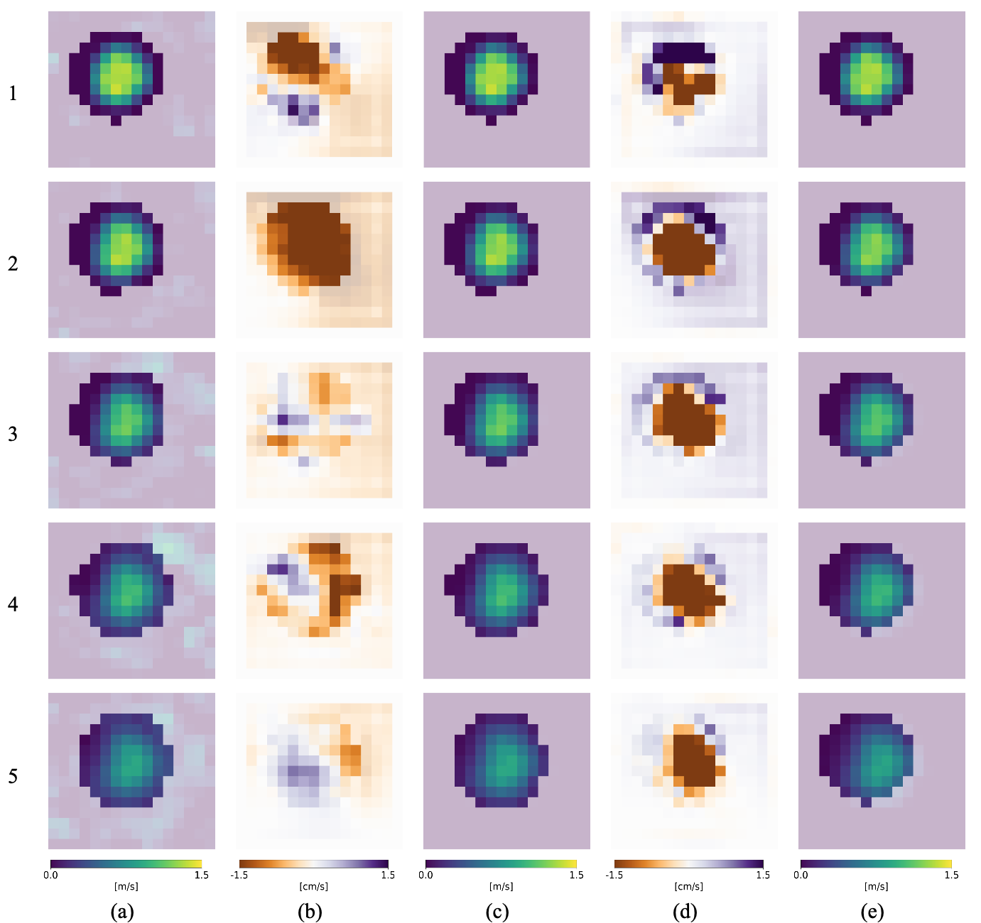
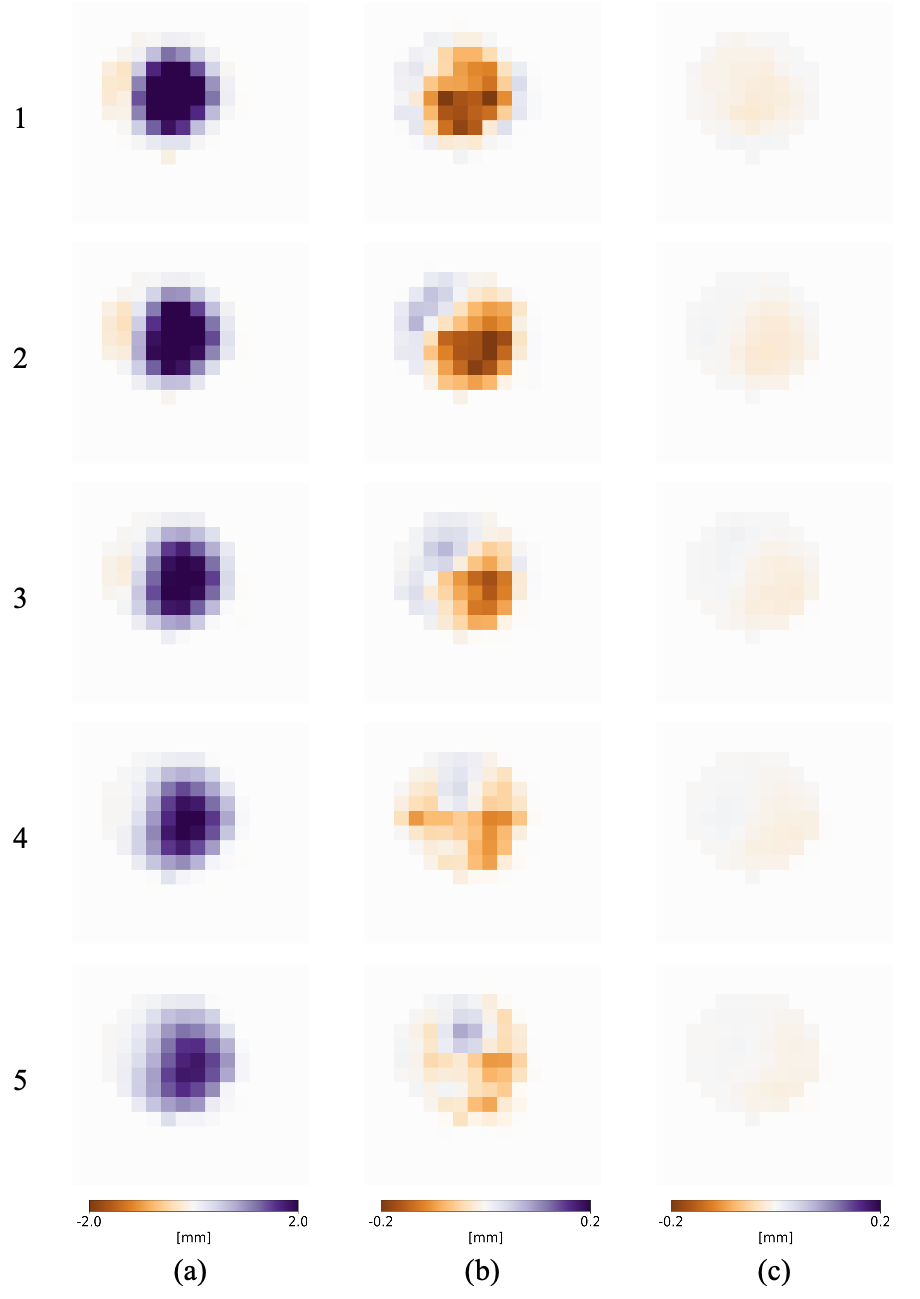
Figure 1b presents the divergence statistics of the four velocity fields used in this approach: uMRI, u, uMRI,s and us. Figure 1 shows a representation of the phantom geometry, the region of interest used for the analysis and the location of the sections for the results. Figure 3 compares the initial velocity measurements, uMRI with the divergence-free fields without and with spatial artifact correction. The calculated spatial shifts in the three cartesian directions are shown in Figure 4.Discussion
In this work a framework using a variational formulation has been developed to reconstruct divergence-free and displacement-corrected velocity vector fields from 4D PC-MRI . The initial measurements exhibited a divergence up to 16 s-1, which has been corrected using the variational formulation coupled with Lagrangian multipliers. Axial velocity differences were in the range of 1-2%, while for the orthogonal components the magnitude of the correction was on the order of 0.1-0.5%. Correcting spatial displacement artefacts was achieved by estimating the un-displaced position of magnetization using the reconstructed divergence-free velocity field for the backwards propagation path-lines. Figures 3 and 4 show that the correction has a dominant component in the axial direction, up to 2 mm, but it also has a projection, although of much lower amplitude, on the phantom sections.Acknowledgements
No acknowledgement found.References
1. Dyverfeldt P, Bissell M, Barker AJ et al. 4D flow cardiovascular magnetic resonance consensus statement. Journal of Cardiovascular Magnetic Resonance; 2015; 17(72).
2 Loecher M, Kecskemeti S, Turski P. et al. Comparison of divergence-free algorithms for 3D MRI with three-directional velocity encoding. Journal of Cardiovascular Magnetic Resonance; 2012; 14(W64).
3. Vlasenko A, Schnörr C. Physically consistent and efficient variational denoising of image fluid flow estimates. IEE Transactions on Image;2010; 9:586-596.
4. Steinman DA, Ethier R and Rutt BK. Combined analysis of spatial and velocity displacement artifacts in phase contrast measurements of complex flows. Journal of Magnetic Resonance Imaging; 1997; 7:339-346.
5. Brezzi F, Fortin M. Mixed and Hybrid Finite Element Methods. New York: Springer;1991.
6. Alnaes MS, Blechta J, Hake J et al. The FEniCS Project Version 1.5. Archive of Numerical Software; 2015; 3.
7. Logg A, Mardal KA, Wells GN et al. Automated Solution of Differential Equations by the Finite Element Method Springer, 2012.
8. Logg A, Wells GN. DOLFIN: Automated Finite Element Computing. ACM Transactions on Mathematical Software;2010;37.
9. Kirby RC, Logg A. A Compiler for Variational Forms. ACM Transactions on Mathematical Software; 2006;32.
Figures