2260
Limitations of Echo Planar Imaging in PC-MRI of High Flow Regimes1University and ETH Zurich, Zurich, Switzerland
Synopsis
An evaluation of velocity field reconstructions from echo-planar trajectories in PC-MRI relative to ground truth computational fluid dynamics (CFD) data in stenotic high flow regimes is presented. The reconstructed velocity images and variations in spatial resolution resulting from modulation of the Point Spread Function (PSF) are investigated. Significant artifacts and resolution loss of up to factor 8 for EPI in high-flow regimes of 220cm/s are found. In-vitro experiments confirm that depending on the orientation of the main flow direction the reconstructed velocity images differ significantly in regions of high shear or acceleration with implications for in-vivo applications.
Introduction
Fast readout strategies such as Echo Planar Imaging (EPI) (1) have been used to address the issue of long acquisition times in 4D Flow MRI (2). However, previous results for EPI (3,4) suggest that reconstructed images suffer from misregistration artefacts depending on the orientation of the phase encoding direction.The present work proposes a framework utilizing Lagrangian particle tracing (5) to generate simulated PC-MRI data from a numerical phantom using readout trajectories as applied on current MR scanners. Using CFD velocity fields derived from a Reynolds Averaged Navier Stokes (RANS) simulation as ground truth (GT), velocity differences are computed and the modulation of the spatial Point Spread Function (PSF) as a function of velocity is quantified. In addition, EPI and GRE data obtained in an in-vitro flow phantom for different orientations of the phase encoding direction are presented.Methods
In-silico experimentThe simulation framework is depicted in Figure 1. The CFD velocity field of the RANS approach performed on a stenotic U-bend (50% stenosis, parabolic inlet profile 100 cm/s) was used as ground truth data for MRI simulations. The maximum velocity downstream of the stenosis was set to 220cm/s. N = 10771 particles were seeded uniformly throughout the geometry at $$$\vec{r}(t_0) = \vec{r}_0 $$$ with $$$ t_0 $$$ being the beginning of the shot. The state vector equation is given as $$\dot{\vec{x}}_i (t) = \begin{bmatrix}\dot{\vec{r}}_i (t) \\ \dot{\varphi}_i(t)\end{bmatrix} = \begin{bmatrix}\vec{v} (\vec{r}_i(t)) \\ \gamma \vec{G}(t) \cdot \vec{r}_i(t) \end{bmatrix}$$ where $$$\vec{\rho}_i(t)$$$,$$$\vec{v}(\vec{r}_i(t))$$$,$$$\varphi_i(t)$$$ and $$$\vec{G}(t)$$$ describe a particle’s position, the CFD velocity field interpolated at the given position, particle’s phase and the magnetic field gradient, respectively. The differential equations were solved for every particle using a Dormand-Prince method in MATLAB (The Mathworks, Natick, MA). At the border of the geometry, particle’s velocities were set to zero to mimic a zero-slip condition.
The trajectories investigated included EPI (5 lines per shot (1)) and GRE, acquiring 1 line per shot. Echo times (TE) and repetition times (TR) were 4ms/6.7ms and 1.8/2.3ms for EPI and GRE, respectively. A Field-of-View (FOV) of 10x10cm2 with a resolution of 1x1mm2 was simulated. The first moment of the bipolar gradient was calculated according to an encoding velocity venc of 500cm/s.
The PSF was assessed by a Gaussian fitting approach which also enabled the characterization of non-sinc PSFs. A proton density image was reconstructed for each particle i={1, 2, …, N} and zero-padded to 5-fold matrix size. In an optimization process, a 2D Gaussian function was fitted to the image, which resulted in parameter $$$\sigma_1$$$ and $$$\sigma_2$$$ which provided the relative broadening of the PSF as $$$\sigma = \frac{1}{\sqrt{\Delta x^2 \Delta y^2}} \sqrt{\sigma_1^2 + \sigma_2^2}$$$ and were used to characterize the effective resolution.
In-vitro experiment
A steady flow phantom (6) was driven by a centrifugal pump. 4D Flow MRI data was acquired on a 3T Philips Ingenia system (Philips Healthcare, Best, the Netherlands) using EPI and GRE readout. Encoding velocity was set to venc =150cm/s per axis and an additional reference measurement with venc=0cm/s. A 32-channel receiver coil was used and data was reconstructed using MRecon (Gyrotools LLC, Winterthur, Switzerland).
Results
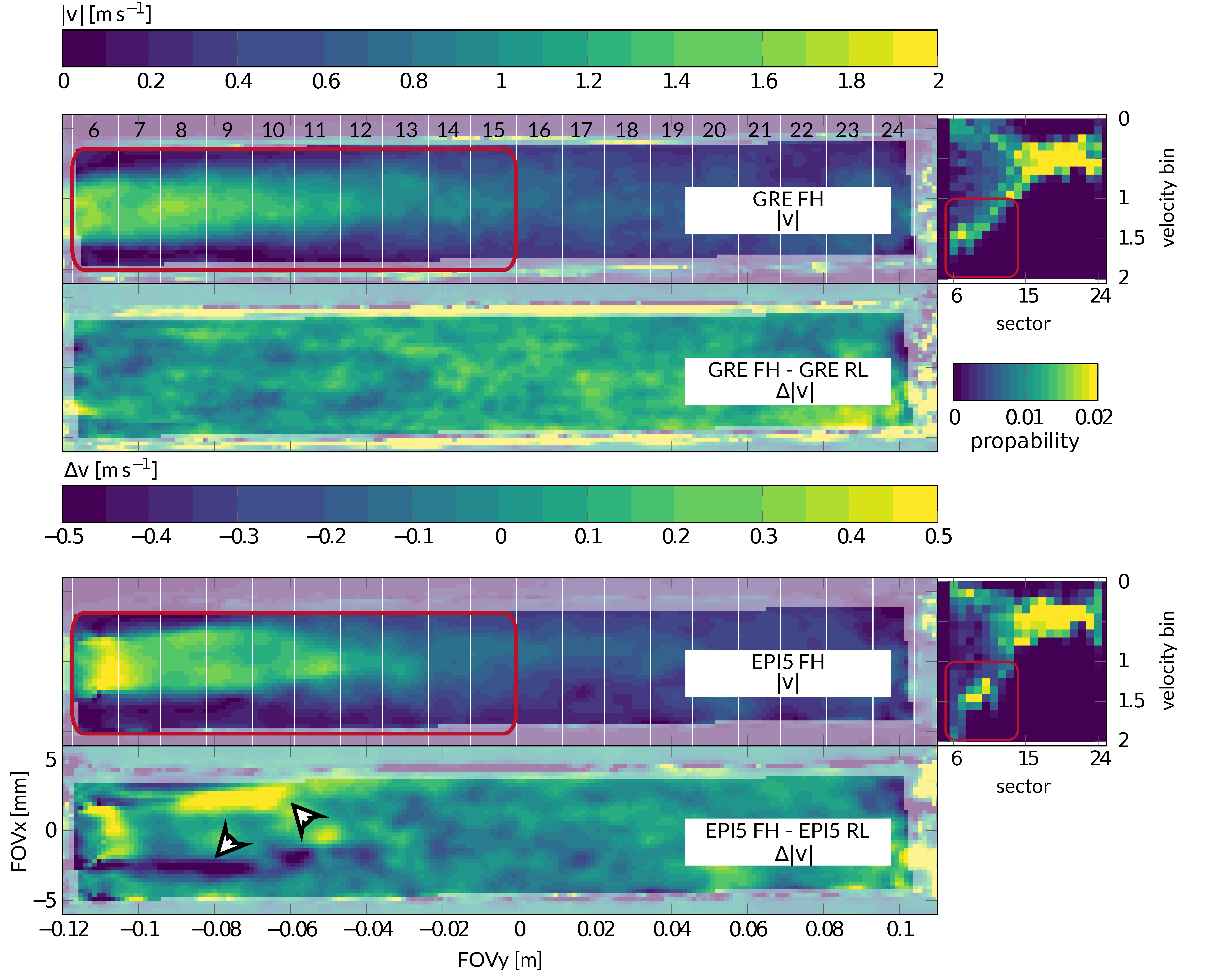
Exemplary particle PSFs for GRE and EPI are shown in Figure 2. Reconstructed velocity images for the in-silico experiment are depicted in Figure 3 for both the phase and frequency encoding direction aligned with the main flow, respectively. A maximum velocity error of 480cm/s for EPI relative to GT was detected in regions of high flow. In contrast to EPI, velocities from GRE did not depend on the orientation within the FOV. Moreover, the PSF of EPI was found to vary significantly as a function of velocity. For GRE, the PSF broadening was 1.3x compared to acquisition resolution, while, for EPI, PSF broadening of factors of up to 8 were measured. Results for the in-vitro experiment can be found in Figure 4. When comparing velocities, a mean velocity differences of 12cm/s and 10cm/s for EPI5 and GRE were obtained.Discussion
In this work, EPI PC-MRI has been investigated under high flow condition. Using a particle tracing approach, simulated data was generated. Using PSF analysis, significant modulation of the PSF in EPI depending on the velocity field with potential impact on quantitative flow metrics was measured. In-vitro data confirmed the orientation dependency of EPI. The jet shape and length was altered when comparing EPI scans with orthogonal phase-encode directionsConclusion
The proposed work demonstrates that phase-contrast MRI of high-flow regimes using EPI readout does result in image artifacts and spatially varying degradation of resolution. Accordingly, a careful selection of acquisition protocols for 2D and 4D Flow MRI of high flow conditions is required in practice.Acknowledgements
No acknowledgement found.References
1. Garg P, Westenberg JJM, van den Boogaard PJ, et al. Comparison of fast acquisition strategies in whole-heart four-dimensional flow cardiac MR: Two-center, 1.5 Tesla, phantom and in vivo validation study. J. Magn. Reson. Imaging 2018;47:272–281 doi: 10.1002/jmri.25746.
2. Dyverfeldt P, Bissell M, Barker AJ, et al. 4D flow cardiovascular magnetic resonance consensus statement. J. Cardiovasc. Magn. Reson. 2015;17:1–19 doi: 10.1186/s12968-015-0174-5.
3. Nishimura DG, Irarrazabal P, Meyer CH. A Velocity k space Analysis of Flow Effects in Echo Planar and Spiral Imaging. Magn. Reson. Med. 1995;33:549–556 doi: 10.1002/mrm.1910330414.
4. Butts K, Riederer SJ. Analysis of flow effects in echo-planar imaging. J. Magn. Reson. Imaging 1992;2:285–93.
5. Petersson S, Dyverfeldt P, Gårdhagen R, Karlsson M, Ebbers T. Simulation of phase contrast MRI of turbulent flow. Magn. Reson. Med. 2010;64:1039–1046 doi: 10.1002/mrm.22494.
6. Binter C, Knobloch V, Manka R, Sigfridsson A, Kozerke S. Bayesian multipoint velocity encoding for concurrent flow and turbulence mapping. Magn. Reson. Med. 2013;69:1337–1345 doi: 10.1002/mrm.24370.
Figures
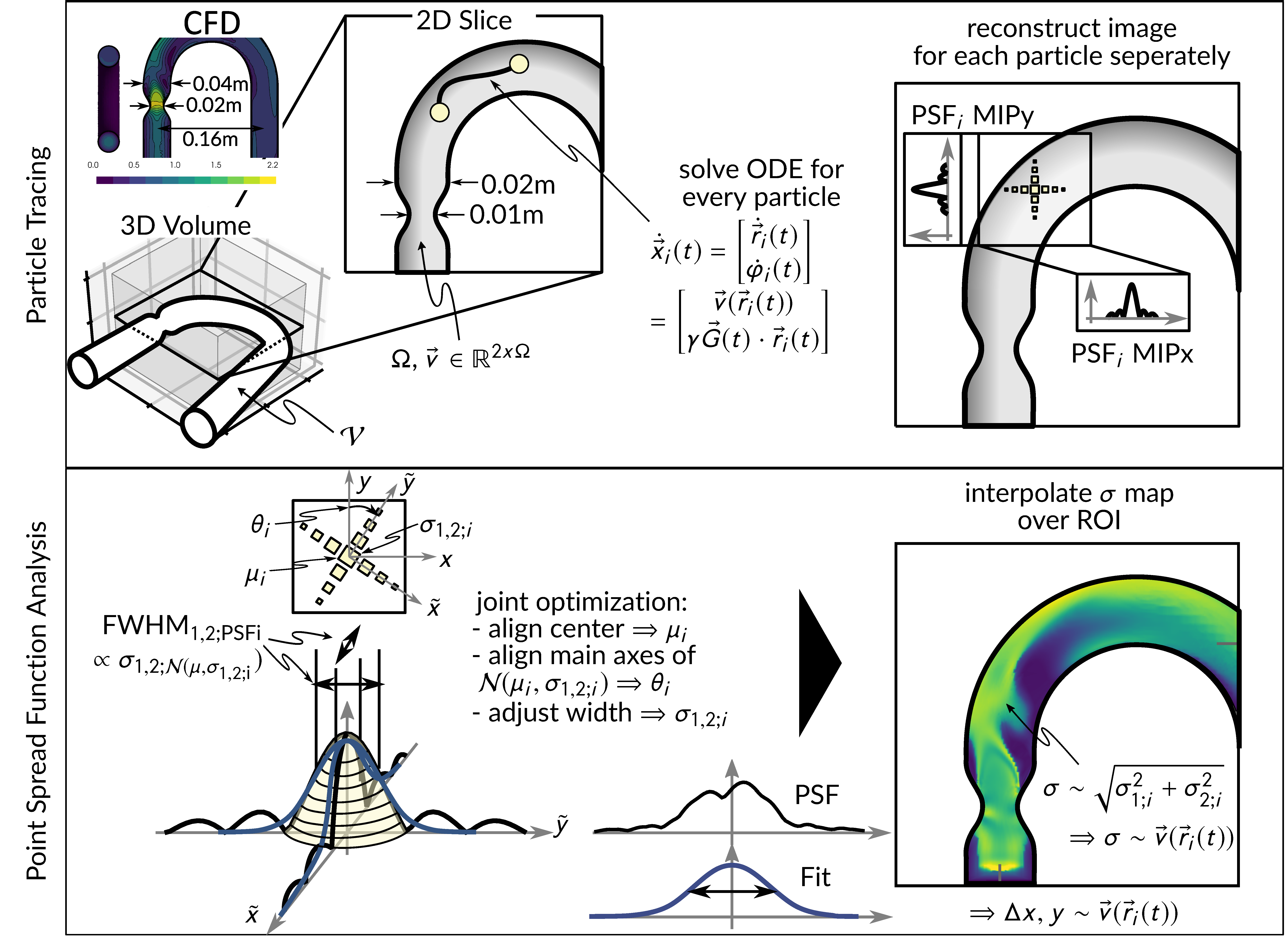
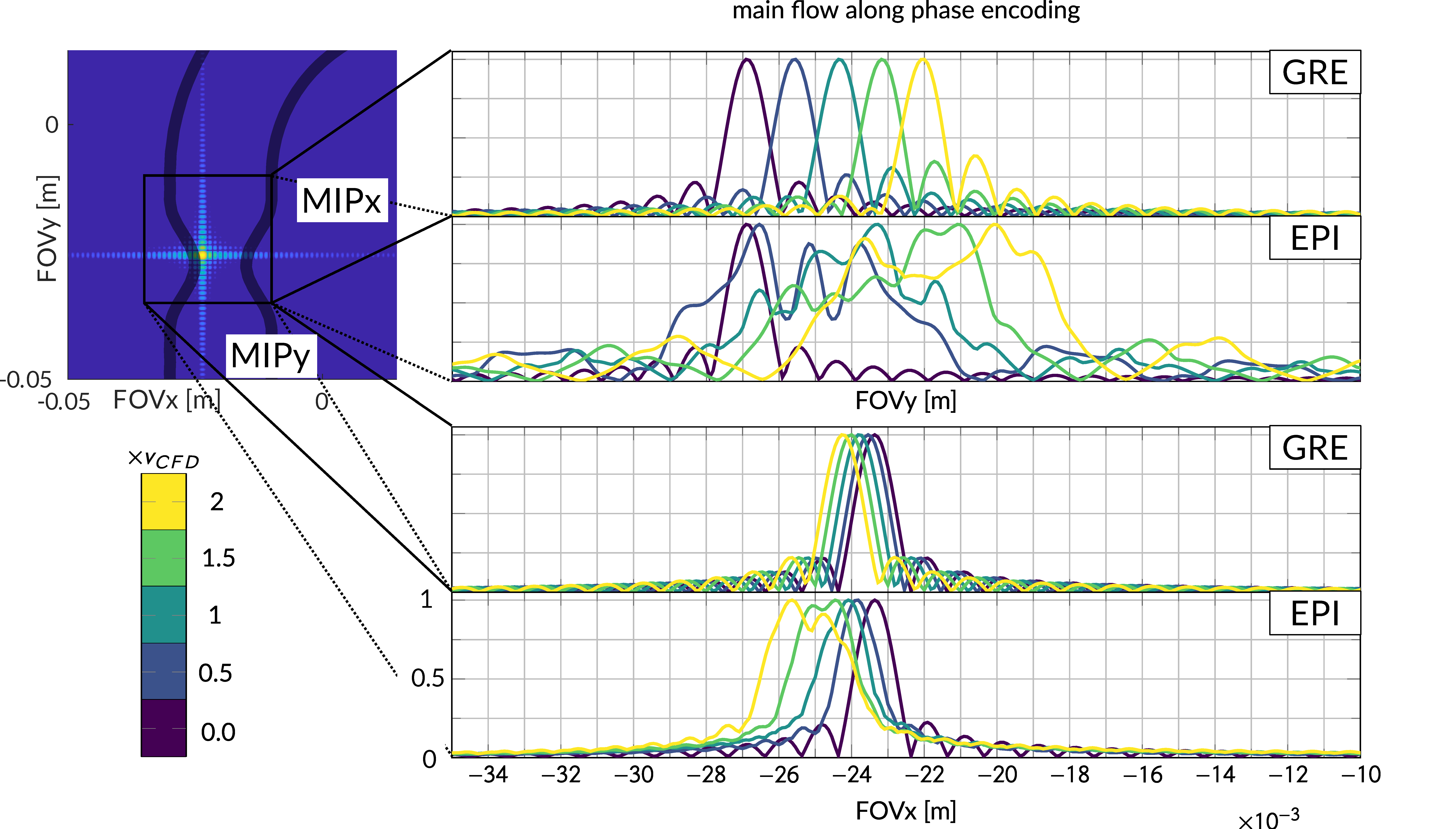
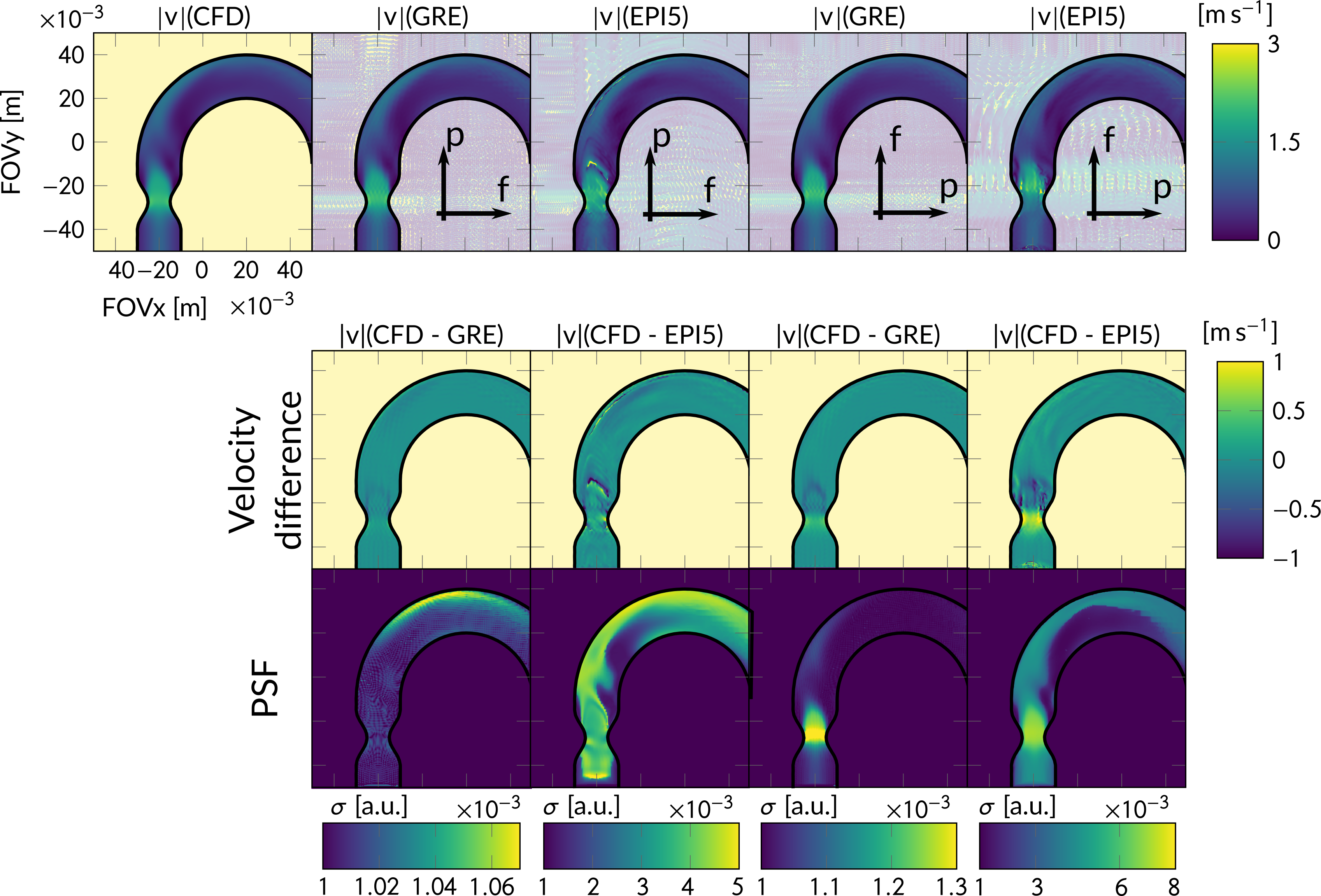
Figure 3: Reconstructed velocity images for the in-silico experiment. f and p denote the frequency and phase encoding direction, respectively. Flow magnitude |v| = √(vx2 + vy2) is presented and difference images |v|(CFD – GRE/EPI5) show over- and underestimation for positive and negative values respectively. Artefacts for EPI5 are pronounced in regions of high shear at the jet border.