2257
On the dynamic range of Reynolds stress tensor quantification1Medical Physics in Radiology, German Cancer Research Center (DKFZ), Heidelberg, Germany, 2Institute of Fluid Mechanics, University of Rostock, Rostock, Germany, 3Physikalisch-Technische Bundesanstalt (PTB), Braunschweig and Berlin, Germany
Synopsis
In this work, we successfully quantified the Reynolds stress tensor (RST) in a well-known fluid-dynamic test case: the flow over periodic hills. This test case was chosen because the turbulence in this kind of flow is strongly inhomogeneous and anisotropic, representing a challenging measurement task. The results indicate, in analogy to intravoxel velocity standard deviation (IVSD) mapping, that RST quantification is highly susceptible to the applied $$$m_1^{enc}~$$$value. Furthermore, RST mapping inherently requires a higher dynamic range compared to IVSD mapping, since the shear stresses are typically much lower than the normal stresses.
Introduction
The relationship between the first gradient moment m1 and the signal phase is used in flow MRI to quantify mean velocities in each voxel. Additionally, the velocity-encoding-related signal loss can be used to characterize turbulence1-3 and to quantify the Reynolds stress tensor (RST)4, a fluid-dynamic parameter that characterizes the turbulent fluctuations in fluid momentum that might be of clinical interest in pathologies with altered hemodynamics. For intravoxel velocity standard deviation (IVSD) mapping, i.e. the quantification of the RST’s diagonal elements, it has been reported that the choice of m1 influences the quantified turbulence3, since low m1 values lead only to insignificant signal loss, whereas large m1 values result in strong signal dephasing such that magnitude images reflect the noise floor. The same problem exists for the quantification of the RST. Here, the normal stresses (diagonal elements) are typically substantially higher than the shear stresses (off-diagonal elements), which requires a high dynamic m1 range to correctly quantify the full tensor.In this work, we examined a well-known fluid-dynamic test case, the flow over periodic hills. This test case was chosen because the turbulence in this flow is strongly inhomogeneous and anisotropic, representing a challenging measurement task.
Theory
Assuming a Gaussian intra-voxel velocity distribution, the corresponding magnitude of an m1-encoded MRI signal can be expressed as:$$\left|S\left(\vec{k}_v\right)\right|=\left|S_0\right|\cdot\exp\left(-\frac{1}{2}\vec{k}_v~\Sigma^{-1}~\vec{k}_v\right)$$
where$$$~\vec{k}_v=\gamma\left[m_{1,x}~m_{1,y}~m_{1,x}\right]^{T}$$$, $$$\gamma$$$ the gyromagnetic ratio, $$$\Sigma$$$ the variance of the 3-dimensional Gaussian, and $$$S_0$$$ the signal of a velocity-compensated measurement.
Multiplying $$$\Sigma^{-1}~$$$by the fluid density $$$\rho~$$$is equal to the RST $$$\tau$$$. Typically, $$$\tau~$$$is obtained by fitting a 3-dimensional Gaussian to the data of six velocity-encoded measurements4 with the following encoding matrix $$$E$$$, according to the ICOSA65 encoding scheme and an additional compensated measurement:
$$E=m_1^{enc}\cdot\begin{bmatrix}0&0&0\\1/sqrt\left(1+\psi^2\right)&0&\psi/sqrt\left(1+\psi^2\right)\\1/sqrt\left(1+\psi^2\right)&0&-\psi/sqrt\left(1+\psi^2\right)\\\psi/sqrt\left(1+\psi^2\right)&1/sqrt\left(1+\psi^2\right)&0\\-\psi/sqrt\left(1+\psi^2\right)&1/sqrt\left(1+\psi^2\right)&0\\0&\psi/sqrt\left(1+\psi^2\right)&1/sqrt\left(1+\psi^2\right)\\0&-\psi/sqrt\left(1+\psi^2\right)&1/sqrt\left(1+\psi^2\right)\end{bmatrix}$$
where $$$\psi=\left(1+sqrt\left(5\right)\right)/2~$$$and $$$m_1^{enc}~$$$is the applied encoding moment. These measurements correspond to six points distributed on a shell with radius $$$m_1^{enc}$$$.
Methods
An in-vitro flow test case as shown in Fig.1A was used that consisted of 13 identical consecutive hills with measurements performed between the 10th and 11th hill. Flow rate and temperature were kept constant at 255l/min and 22°C, resulting in a Reynolds number of Re≈60000. Data were acquired on a 3T system (Magnetom Trio, Siemens, Germany) with a custom phase-contrast sequence employing an ICOSA6 encoding with values of [2.5,$$$~$$$5,$$$~$$$10,$$$~$$$15,$$$~$$$20,$$$~$$$25,$$$~$$$30,$$$~$$$35,$$$~$$$40,$$$~$$$45, $$$~$$$50,$$$~$$$60] mT/m·ms². Acquisition parameters: resolution=1.0x1.0x6.0$$$\,$$$mm³, FOV=496x120$$$\,$$$mm², TE/TR=6.32/10.0$$$\,$$$ms, averages=256.For velocity quantification, the phase data were corrected for background phases by additional measurements without flow and averages=4 but otherwise identical settings. The velocity vector field was then reconstructed from the data corresponding to the five lowest $$$m_1^{enc}~$$$values to minimize phase bias from higher orders of motion (e.g. acceleration). The RST was quantified by two different methods. First, by fitting a 3-dimensional Gaussian to the magnitude data of the 12 ICOSA6-encoded measurements, normalized by the velocity-compensated measurements. To avoid the offset due to the Rician nature of the magnitude noise, data points with less than 10% normalized magnitude were excluded from the fit. Second, the RST was calculated by fitting a 3-dimensional Gaussian individually for every $$$m_1^{enc}~$$$value.
Results
The three velocity vector field components shown in Fig.1C illustrate that the velocities are restricted to the x-y plane within the examined slice. Example magnitude images for all 12 shells along the second encoding direction are shown in Fig.2A, demonstrating the high range of turbulence present in the test case. This finding is supported quantitatively by Fig.2B, which displays the measured data of two regions marked in Fig.2A with corresponding Gaussian fits. Note that here, only the projection of the three-dimensional Gaussian along the second encoding direction is shown. Additionally, Fig.2C+D show differences between the Gaussian fit to the full dataset compared to individual Gaussian fits to two example $$$m_1^{enc}~$$$values. In the case of high turbulence (Fig.2D), the individual fit to $$$m_1^{enc}$$$=45$$$\,$$$mT/m·ms² leads to a substantial overestimation of $$$\Sigma~$$$and therefore to an underestimation of the RST (7-fold for$$$~\tau_{xy}$$$).All six components of the RST, quantified by the Gaussian fit to the full dataset, are illustrated in Fig.3A-F. As expected, $$$\tau_{xx}~$$$and $$$\tau_{xy}~$$$are the highest normal and shear stresses with peak values of 6.4$$$\,$$$m²/s² and 3.8$$$\,$$$m²/s² respectively. In contrast, lower shear stresses of 0.7$$$\,$$$m²/s² and -1.0$$$\,$$$m²/s² are obtained for $$$\tau_{xz}~$$$and $$$\tau_{yz}$$$. Additionally, the turbulent kinetic energy (TKE), the trace of the RST (see Fig.3G), yielded peak values of 6$$$\,$$$kJ/m³.
Fig.4+5 display results from the individual Gaussian fits to five example $$$m_1^{enc}~$$$values, indicating amplified noise for low $$$m_1^{enc}~$$$values and peak stress underestimation for high $$$m_1^{enc}~$$$of up to 3-fold for $$$\tau_{xx}~$$$and the highest $$$m_1^{enc}$$$. Furthermore, this method fails to correctly quantify the smallest shear stress components $$$\tau_{xz}~$$$and $$$\tau_{yz}$$$.
Discussion
In this work, we successfully quantified the RST in a well-known fluid-dynamic test case that produces stresses over a high range. However, additional data either from simulations or other reference measurements would be needed to estimate the method’s accuracy. The results indicate, in analogy to IVSD mapping, that RST quantification is highly susceptible to the applied$$$~m_1^{enc}~$$$value. Furthermore, RST mapping inherently requires a higher dynamic range compared to IVSD mapping, since the shear stresses are typically much lower than the normal stresses.We speculate that multiple$$$~m_1^{enc}~$$$values are in general necessary to correctly quantify all components of the RST, not only for this particular test case.
Acknowledgements
No acknowledgement found.References
1. Dyverfeldt, P. , Sigfridsson, A. , Kvitting, J. E. and Ebbers, T. (2006), Quantification of intravoxel velocity standard deviation and turbulence intensity by generalizing phase‐contrast MRI. Magn. Reson. Med., 56: 850-858. doi:10.1002/mrm.21022
2. Dyverfeldt, P. , Kvitting, J. E., Sigfridsson, A. , Engvall, J. , Bolger, A. F. and Ebbers, T. (2008), Assessment of fluctuating velocities in disturbed cardiovascular blood flow: In vivo feasibility of generalized phase‐contrast MRI. J. Magn. Reson. Imaging, 28: 655-663. doi:10.1002/jmri.21475
3. Dyverfeldt, P. , Gardhagen, R. , Sigfridsson, A. ,Karlsson, M. and Ebbers, T. (2009), On MRI turbulence quantification. Magn. Reson. Imaging, 27:913-922. doi:10.1016/j.mri.2009.05.004
4. Haraldsson, H. , Kefayati, S. , Ahn, S. , Dyverfeldt, P. , Lantz, J. , Karlsson, M. , Laub, G. , Ebbers, T. and Saloner, D. (2018), Assessment of Reynolds stress components and turbulent pressure loss using 4D flow MRI with extended motion encoding. Magn. Reson. Med, 79: 1962-1971. doi:10.1002/mrm.26853
5. Hasan, K. M., Parker, D. L. and Alexander, A. L. (2001), Comparison of gradient encoding schemes for diffusion‐tensor MRI. J. Magn. Reson. Imaging, 13: 769-780. doi:10.1002/jmri.1107
Figures
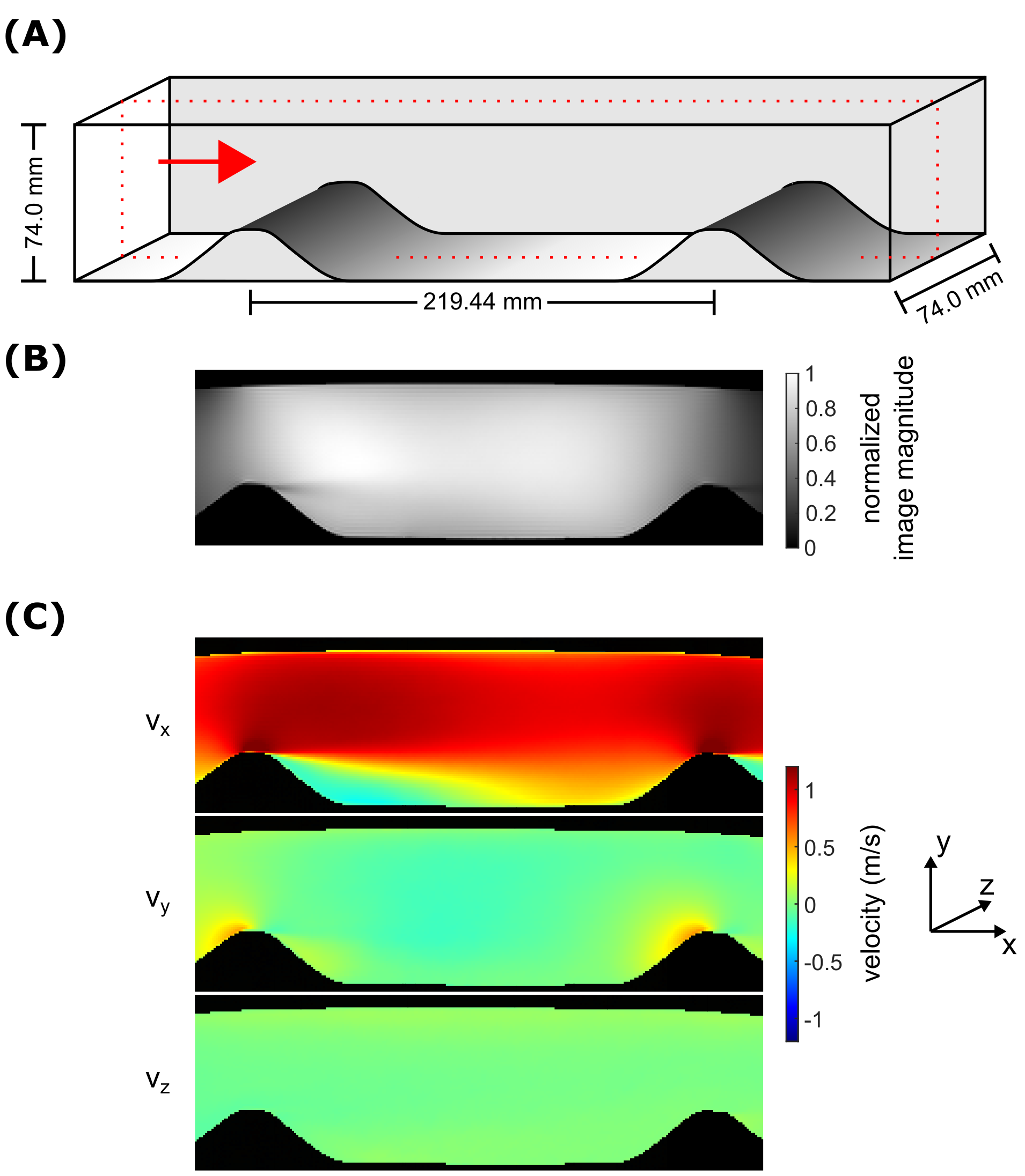
Figure 1:
A) Schematic of the phantom with flow direction indicated by the red arrow. B) Normalized image magnitude and C) velocity components reconstructed from the data corresponding to the five lowest $$$m_1^{enc}~$$$values, with slice positioning corresponding to the dashed red rectangle in A).
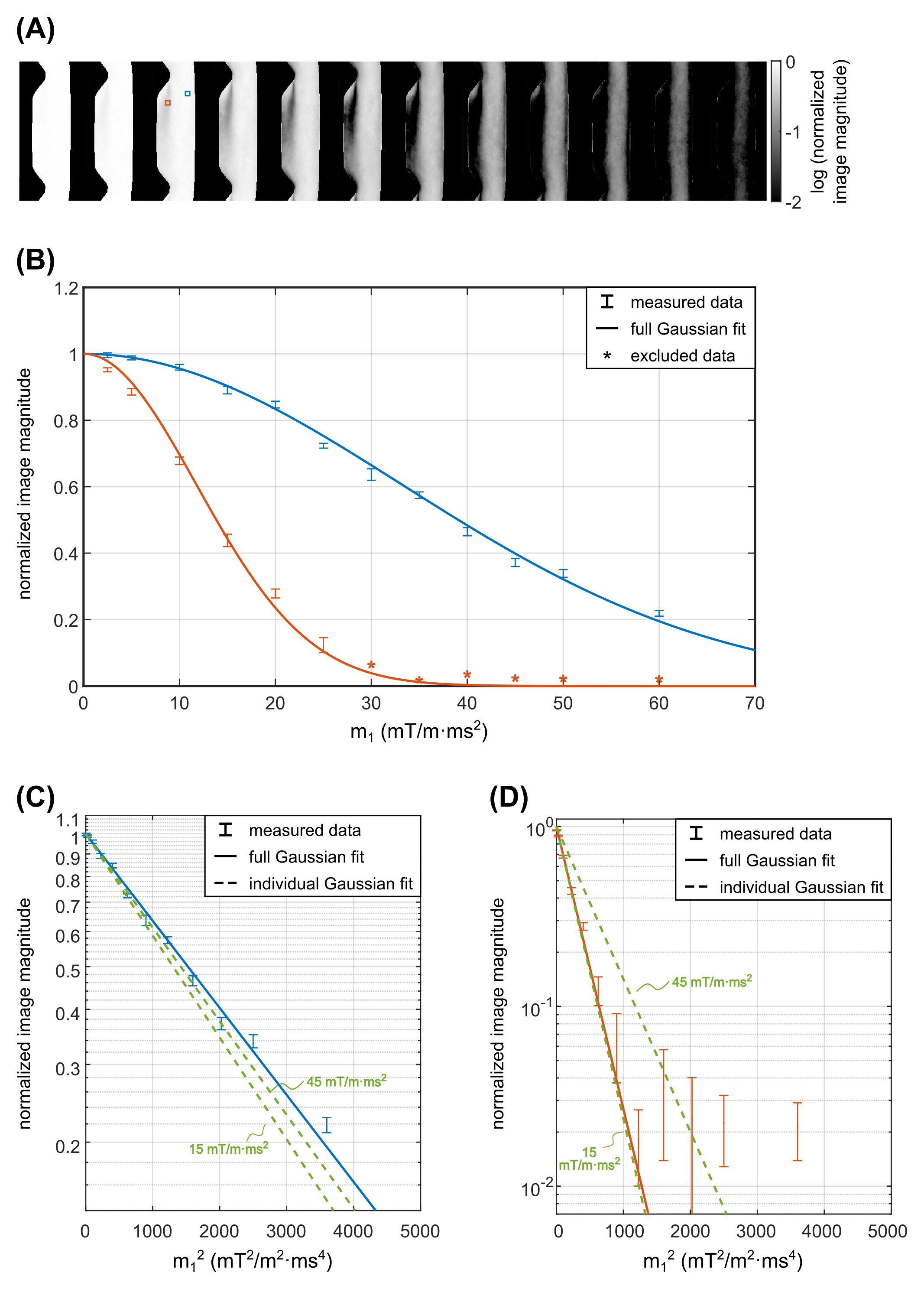
Figure 2:
A) Logarithm of the normalized image magnitude, corresponding to the 2nd encoding direction for all $$$m_1^{enc}~$$$values. B) Gaussian fit to the full data set in the two example voxels marked in A). Data points marked by an asterisk are excluded from the reconstruction. C+D) Comparison between the full Gaussian fit and the individual Gaussian fit for example $$$m_1^{enc}~$$$values of 15 and 45 mT/m·ms² for the two different voxels.
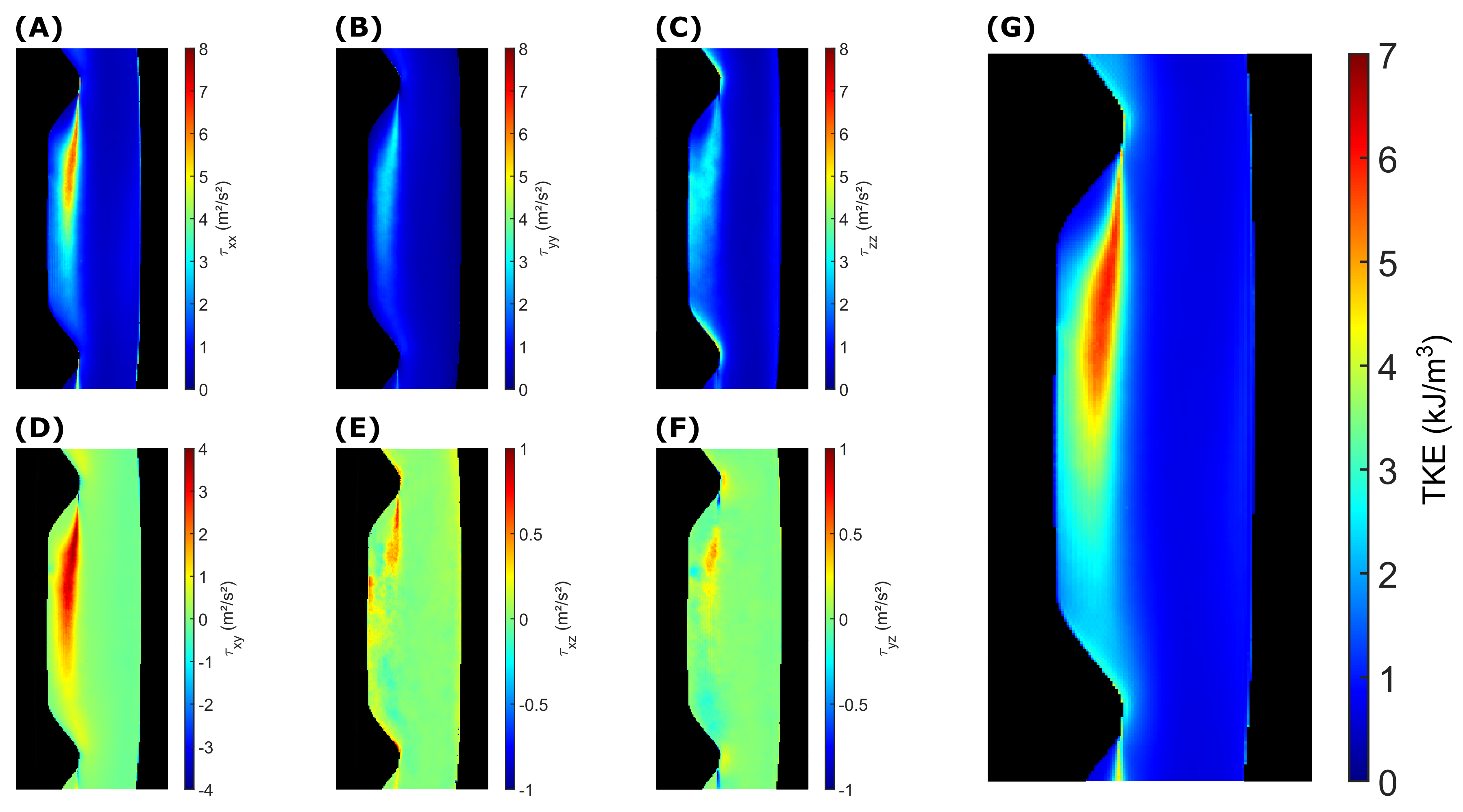
Figure 3:
A)-F) Calculated Reynolds stress tensor components obtained from the Gaussian fit to the full dataset. Note that the scales are not identical for each component. G) Turbulent kinetic energy (TKE), given by the trace of the Reynolds stress tensor, with peak values of 6$$$\,$$$kJ/m³.
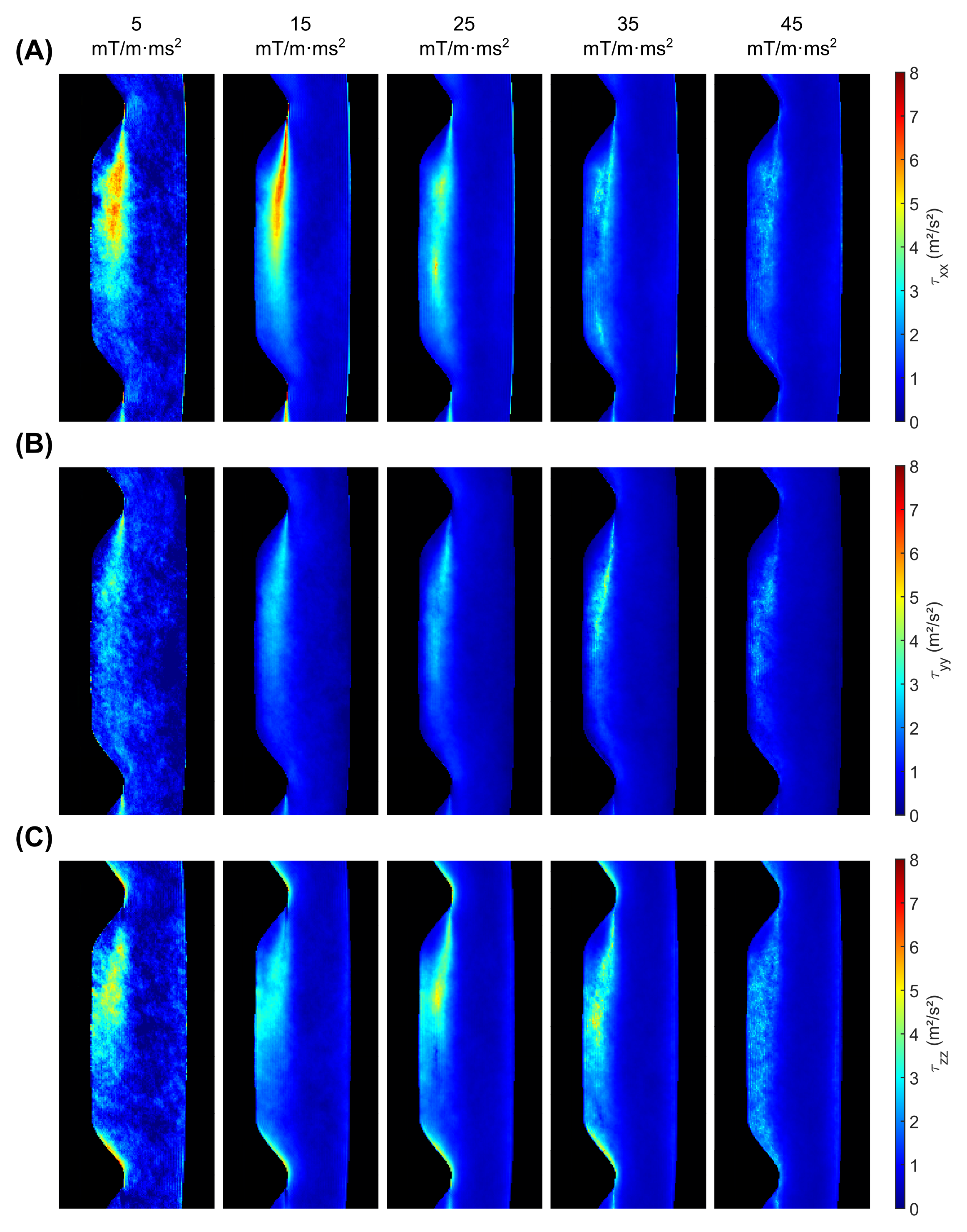
Figure 4:
Normal stresses obtained from the linearized fit for different $$$m_1^{enc}~$$$values of [5, 15, 25, 35, 45] mT/m·ms². While too low $$$m_1^{enc}~$$$values lead to enhanced noise, large $$$m_1^{enc}~$$$values lead to a substantial underestimation of the peak stress of up to 3-fold for $$$\tau_{xx}$$$.
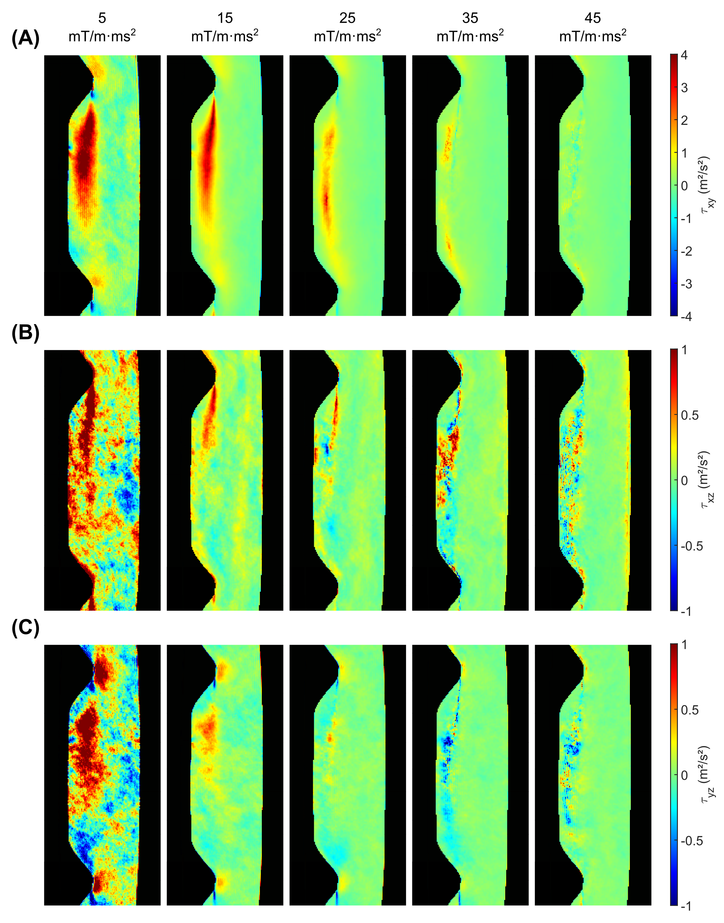
Figure 5:
Shear stresses obtained from the linearized fit for different $$$m_1^{enc}~$$$values of [5, 15, 25, 35, 45] mT/m·ms². High $$$m_1^{enc}~$$$values lead to a substantial underestimation of the peak stress of up to 7-fold for $$$\tau_{xy}$$$. The small shear stresses $$$\tau_{xz}~$$$and $$$\tau_{yz}~$$$are not correctly resolved for any of the $$$m_1^{enc}~$$$values.