Introduction

Radiologic diagnosis of cardiac MRI data is often made based on the 16- (or 17-) segment myocardial model.¹ The degree and characteristic of myocardial contractility, ischemia, and viability (measured by cine, perfusion, and late gadolinium enhancement (LGE) sequences, respectively) depend on the location in the myocardium and are described based on the 16- (or 17-) segment myocardial model by cardiac radiologists. Recent advancement of deep learning in cardiac MRI analysis² led to accurate and automatic quantification of ejection fraction and wall thickness, but for learning, it requires manual contouring/labeling on cardiac images, which is tedious and time consuming. This study focused on the development of deep learning without substantial manual labeling to automatically classify late enhancement lesions, based on the 16-segment model.

Methods

Image Acquisition
A total of 66 subjects, who had cardiac LGE exams at 1.5 Tesla, were considered for this study. Of the 66 subjects, 25 suffered from coronary artery disease (CAD), 25 had hypertrophic cardiomyopathy, and 16 had aortic stenosis. In LGE, an inversion time (TI) scout scan was performed to optimize the inversion time for effective nulling of the healthy myocardium. After the choice of inversion time, 9-10 short-axis slices were acquired during breath-holds in diastole, 15 min after a bolus injection of the contrast agent. An inversion recovery sequence was used for magnetization preparation, and a balanced SSFP sequence was used for the readout. Imaging parameters were as follows: slice thickness = 6 mm, TE = 1.2 ms, TI = 280 - 360 ms, FOV = 400 x 362 mm², image matrix = 256 x 232, pixel size = 1.56 x 1.56 mm², and spacing between slices = 10 mm.

Data Processing
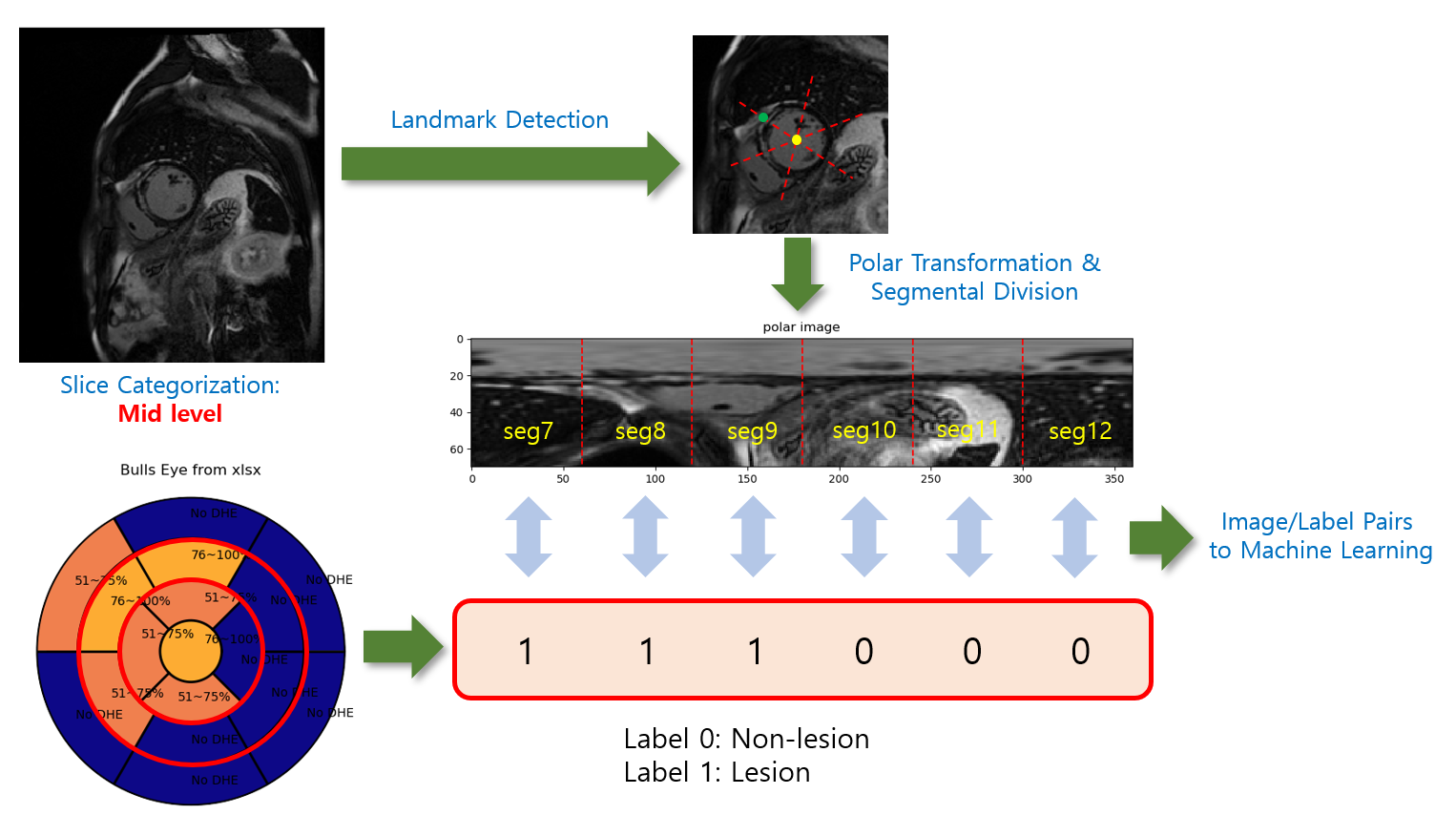
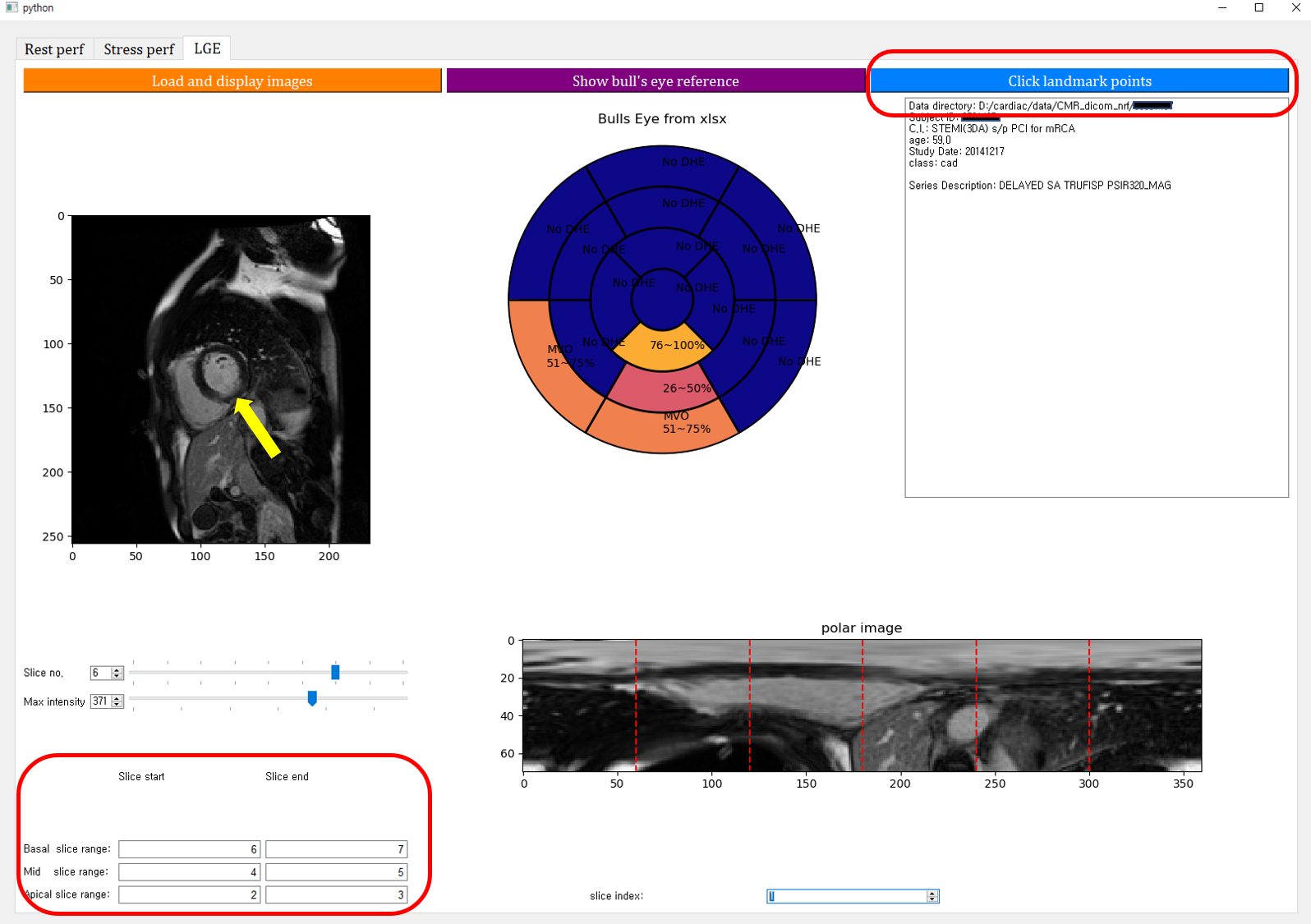
Figure 1 illustrates a flowchart of the proposed data processing scheme. Radiologic diagnosis results were saved in a Microsoft Excel spreadsheet, where 0 stands for non-lesion, 1 for 1~25% of subendocardial enhancement, 2 for 26~50%, 3 for 51~75%, 4 for 76~100%, N for non-ischemic pattern, and M for mid-layer enhancement. A custom Python graphical user interface (shown in Figure 2) was developed to (1) load the spreadsheet information and display it on a color-coded bull’s eye plot, (2) categorize the LGE slices into apical, mid, and basal levels, (3) locate the left ventricular (LV) center point and the anterior right ventricular (RV) insertion points in the slices of interest, and (4) transform images to polar space and save the polar transformed images and their associated diagnosis results for machine learning.

Model Development
Polar image dimensions were 70 x 60 for basal and mid slice images and 70 x 90 for apical slice images. The images were resized to 128 x 128 for model training. In this study, we labeled non-lesion cases as 0 and labeled lesion cases (including subendocardial enhancement, non-ischemic pattern, and mid-layer enhancement) as 1. The CNN model was developed for training in Keras and had four convolutional layers/ReLu activation layers/Max pooling layers, followed by a fully connected layer of 8192 x 64, drop-out with rate = 0.5, and softmax activation. Adam optimization with learning rate = 0.000001 and binary cross-entropy were used for training. Model training and validation accuracy results were obtained at each epoch, up to 100 epochs. The total of polar segmental images was 2,112. The number of training images was 1,690, while the number of validation images was 422.

Results

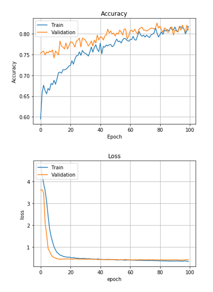
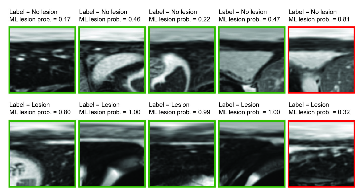
As shown in Figure 3, the learning curves for accuracy and loss appeared stable without any significant degree of overfitting up to the 100th epoch. Training and validation accuracy results were similar (> 0.80). Some sample image classification results from validation datasets are shown in Figure 4, with a machine learning predicted probability score on top of each image. The green rectangles indicate correctly predicted cases, while the red rectangles indicate incorrectly predicted cases. The myocardial band in the images labeled as lesion (bottom row of Figure 4) appears heterogeneous and bright, while the images labeled as non-lesion (top row of Figure 4) show homogeneous and dark patterns in the myocardial band.

Discussion

This study demonstrates that segmental diagnosis results assessed by cardiac radiologists can be used as output labels for supervised model training, along with segmental polar-transformed images. In the current implementation, slice categorization and landmark detection were manually performed, but these processes can be automated using machine learning.^3,4

Lesions may be overlapped between adjacent segments although radiological evaluations indicate that only one segment is labeled as lesion. In this case, it may be necessary to correct radiological evaluation results. This study only focused on a simple task of binary classification (i.e., lesion vs. non-lesion). It is noted that there are different types of lesion characteristics (for example, need for a differentiation of < 25% subendocardial lesion from > 75% subendocardial lesion). More subtle differentiation of lesion characterization may require multi-class classifier CNN models, and the development/validation of the models remain as future work.

Conclusion

The proposed method does not require manual delineation of late gadolinium enhanced lesions for CNN model training and demonstrates a segmental lesion/non-lesion classification accuracy of 0.80.

Acknowledgements

This work was supported by the Basic Science Research Program through the National Research Foundation of Korea (NRF-2018 R1D1A1B07042692).