Introduction

Deep learning has been greatly successful in many areas and is rapidly replacing algorithm-based methods. In medical field, applications were more limited than in other areas due to restricted accessibility of bio-medical data or images. In this regard, transfer learning can be a choice to add similar data for pre-learning of the neural network.¹ Performance and characteristics of the neural network with transfer learning standalone learning are compared and analyzed by learning curves, patterns in multi-layers of the neural networks, and reconstructed image quality.

Methods

An open database for cardiovascular CINE images from York University (denoted as “Y-data”) was used for ‘pre-learning.’² Total 5220 images of 32 subjects were used (22 subjects for training and 10 for test). For ‘main-learning’ (or fine-tuning) cardiac CINE MRI were measured without compression from 3.0T MRI system (Siemens) using balanced-SSFP method for eight volunteers (denoted as “K-data”).³ Total 2016 images were used (4 subjects for training and 4 for test). Both data have short axial views and are assumed to be ground truth images. By computer simulation, compressed data were generated in k-space by subsampling the data with compression ratio of 2, 3, 4, and 8. A single neural network was constructed for the compressed data. An initial reconstruction of compressed-sensing data is achieved by filling the missing data with linear interpolation of the measured data in adjacent frames and applying a two-dimensional FFT. Normalized initial reconstructed image becomes input to the neural network, and the difference between ground truth image and initial reconstructed image becomes the target image to the neural network after normalization. The neural network is composed of U-net.⁴ The learning process of neural network depends on initial value of weights. In standalone learning, weights are initialized randomly⁵ and in transfer learning, optimized weights from pre-learning are used as initial weights for main-learning.

Results

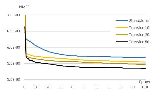
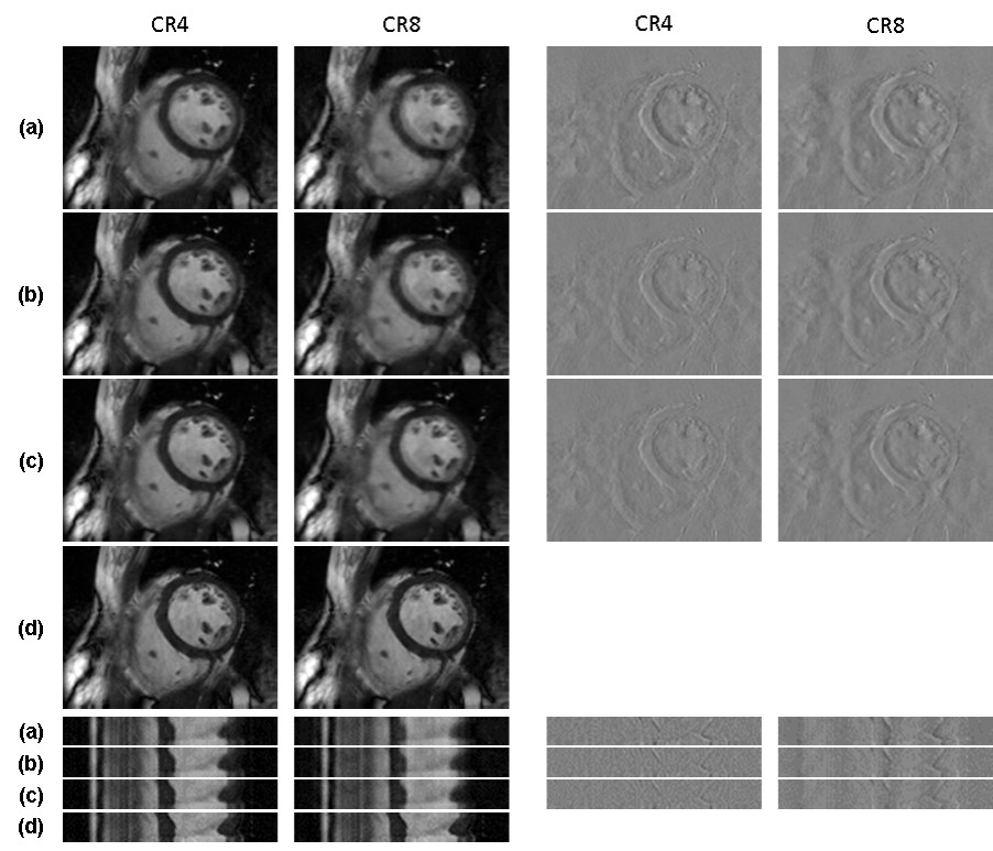
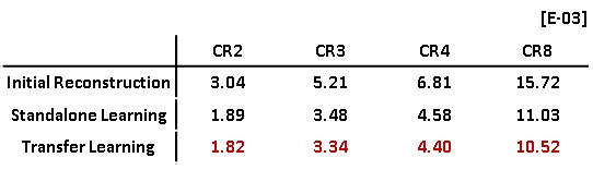
Figure 1 shows the learning curve of neural network according to the weights initialization method. The horizontal axis represents epoch and the vertical axis represents the normalized mean square error (NMSE). A curve for standalone learning and three curves for transfer learning with different amounts of pre-learning are exemplary shown. The amount of pre-learning is defined as the number of epochs used for pre-learning. As shown in Fig.1, NMSEs of transfer learning decreases rapidly compared to standalone learning. For example, NMSEs of transfer learning-10, -20, and -50 with epochs of 20, 5, 2, respectively are lower than that of standalone learning with epoch of 100. This implies 80, 95, and 98 % saving in learning time are achieved by transfer learning Figure 2 is a visualization of the hierarchical layers of the U-net with standalone learning (a) and transfer learning-50 (b). The visualization is the average of the channel outputs. All channel values are non-negative since they go through ReLU after convolution. Transfer learning detects artifacts due to compressed-sensing better than standalone learning as is seen in Fig.2. Figure 3 shows the reconstructed images for the test data using (a) initial reconstruction, (b) deep neural network with standalone learning, (c) deep neural network with transfer learning-50, and (d) ground-truth imaging. The upper left images are the region of interest (ROI) on the transverse plane of reconstruction. ROI covers the entire heart and has a size of 90x120. The lower left images are stack of line profiles alone cardiac phase vertically. On the right are the difference images between the ground truth images and the reconstructed images. The average NMSE for ROI of the test data is summarized in Table.1. As shown as Fig.3 and Table 1, reconstruction by the neural network significantly reduces NMSE compared to the initial reconstruction, and the transfer learning makes the lowest NMSE.

Discussion

Both data of pre-learning and main-learning have short axes views, however, there are many differences. The Y-data for pre-learning are clinical images, while the K-data for main-learning are healthy volunteers’ images. Image quality of Y-data is lower than K-data, presenting aliasing error along phase encoding direction. Despite these differences, a small amount of pre-learning results in improved performance, better generalization, and shorter learning time for main-learning. Thus pre-learning data need not be very similar to the main-learning data. Transfer learning between two much more different data sets is worth trying in the future.

Conclusion

Compressed-sensing cardiovascular CINE MRI was successfully performed by deep artificial neural network with transfer learning. The transfer learning performed better than standalone learning, which helps generalize the neural network even with small learning data. Learning time is also reduced by transfer learning.

Acknowledgements

This work was supported by the National Research Foundation of Korea (NRF) grant funded by the Korea government (MSIP) (NRF-2019R1A2C2005660). The present research has also been conducted by the research grant of Kwangwoon University in 2019.