Introduction

Rapid acquisition and reconstruction techniques are critical for cardiac perfusion MRI. However, the current state of the art methods, such as constrained reconstruction, are able to provide high-quality images from sparsely sampled k-space, though at the cost of slower reconstruction speeds[1]. Such algorithms will take minutes to reconstruct a full dataset, which consists of 2-4 image slices and 70-100 image frames, even when such algorithms are implemented using cutting edge computing techniques. This is problematic from a clinical perspective as it precludes immediate feedback for the scanner operator as to whether the scan quality is sufficient.

Advances in neural networks have provided tools to achieve similar reconstruction quality seen in constrained reconstruction methods, but are computationally much more efficient after the network is sufficiently trained[2]. In this work, we apply deep learning techniques to radially sampled cardiac perfusion MRI datasets and compare reconstruction speeds, image quality, and calculated perfusion index.

Methods

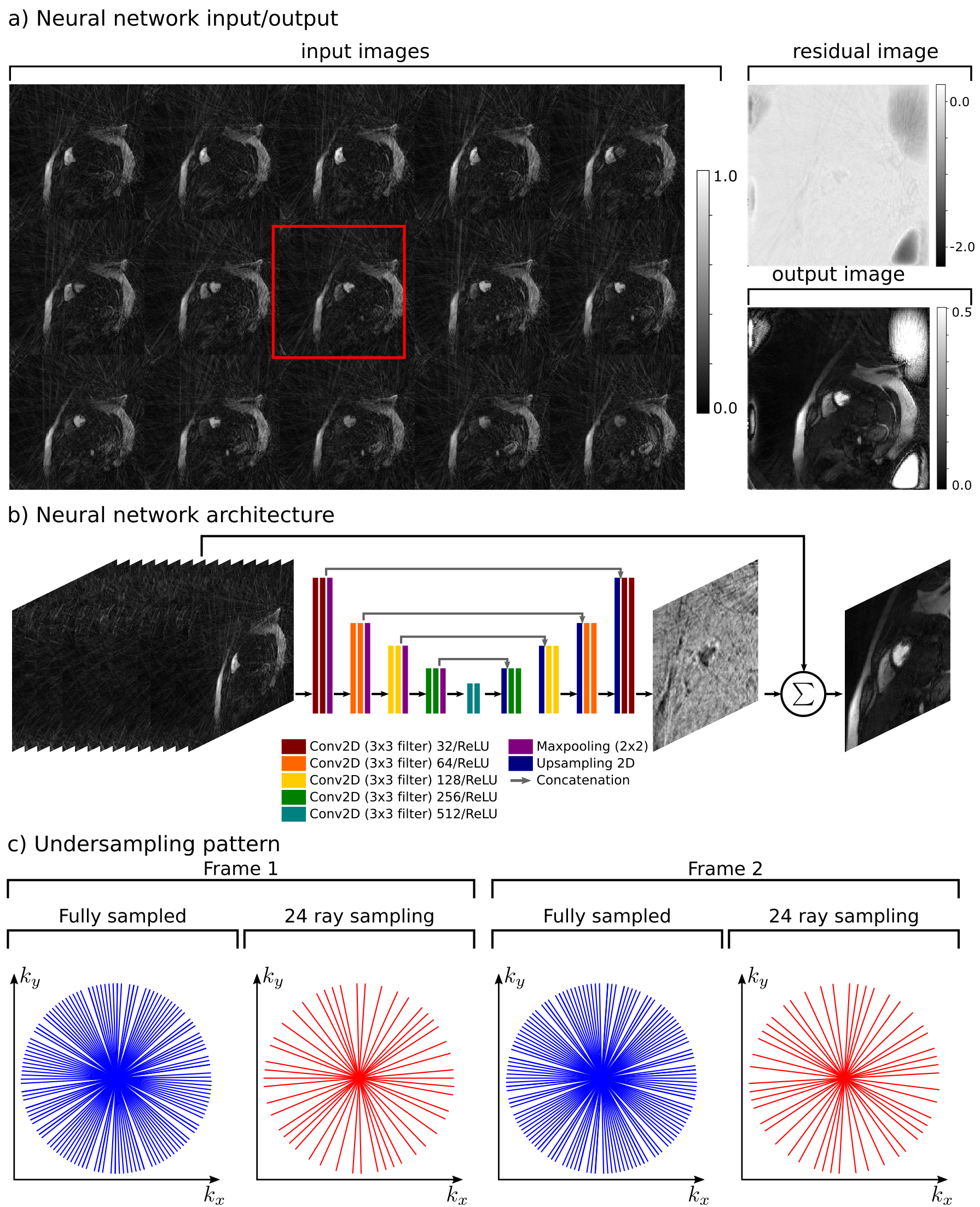
Cardiac perfusion datasets were acquired from thirty participant subjects. All MRI data were acquired using either a Siemens 3T Trio or a 3T Verio scanner using a 12-element phased-array coil. Dynamic contrast-enhanced myocardial perfusion imaging was done first at rest, then during adenosine infusion according to [3]. The contrast was injected approximately 3 minutes after the start of the adenosine infusion and approximately 90 seconds after the regadenoson injection. A saturation recovery radial turboFLASH pulse sequence was used. Seventy-two rays were acquired after each saturation pulse. Additional scan parameters were TR of 2.6 ms, a TE of 1.14 ms, flip angle of 14deg. The voxel size was 2.3x2.3x8mm. Each scan included 2-4 slices acquired for each heartbeat for approximately 1 minute during free breathing.

Data were reconstructed using a neural network architecture operating in the image space. The raw radial k-space data were retrospectively undersampled to 24 rays in a quasi-golden angle fashion. This k-space data were then gridded and transformed to image space using a NUFFT. Magnitude images were fed into the network, which consisted primarily of a U-net[4] architecture. A standard input and output training pair consisted of one slice. On the input, 15 consecutive time frames of the same slice were using and treated as separate channels. The middle channel (in this case, the eighth channel) was considered to represent the target time-frame. On the output, a single channel final image was produced. Fig.1 includes the input/output relationship of this network, the network architecture, and sampling pattern. Because each participant was scanned multiple times with multiple injections, and each scan included multiple slices, and each slice was scanned with 60-100 time frames, 10700 training samples along with 2300 validation samples were used to train the network.

Data from three separate study participants (for a total of ten total injections) were withheld from model training and validation as test data. These images processed by the neural network were benchmarked by comparing them to images reconstructed using standard iterative techniques using the full 72 rays (considered here to be the reference) and the subsampled 24 rays.

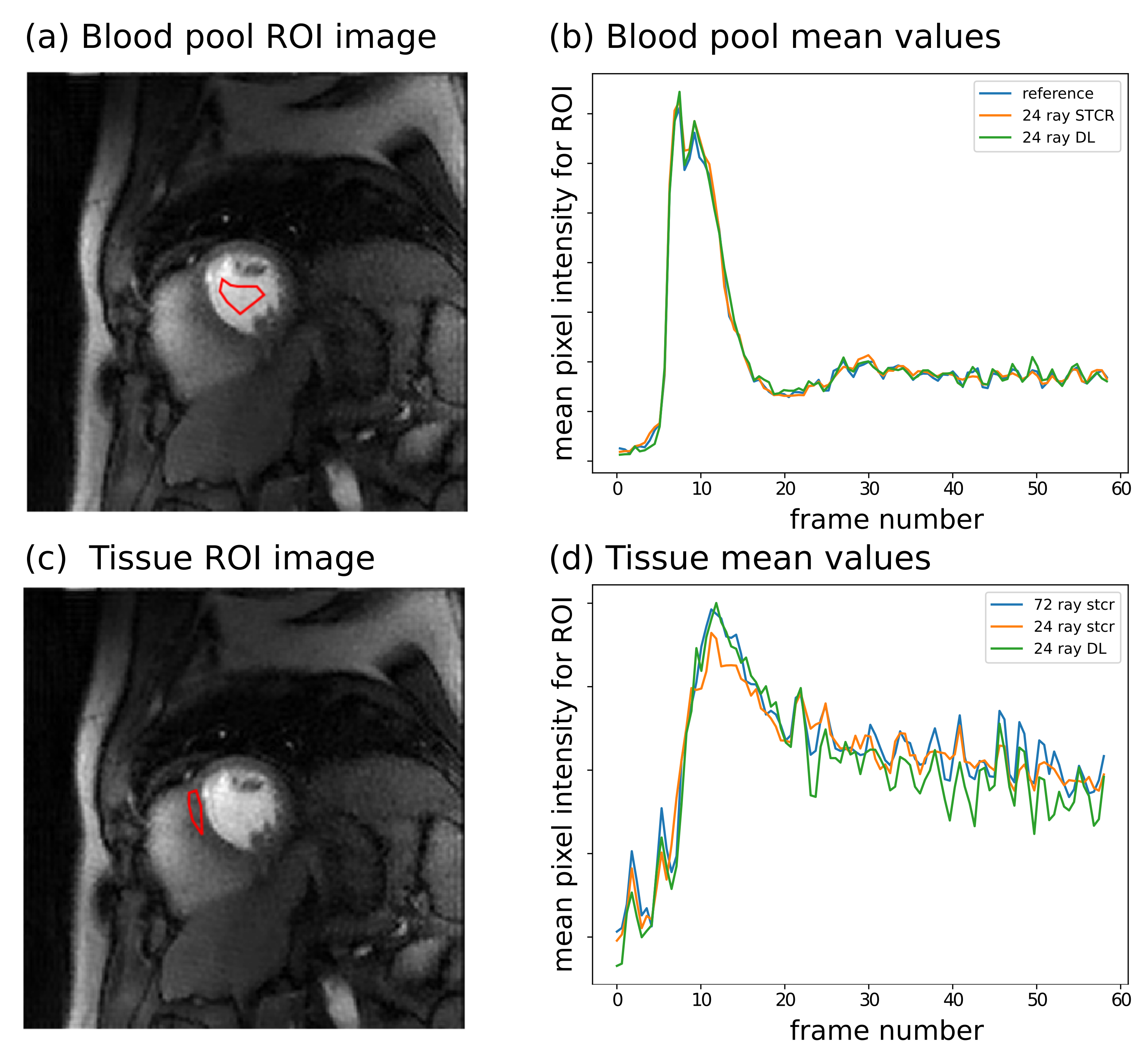
To calculate a perfusion index, images were first registered for inter-frame motion, and then a region of interest in the blood pool and tissue borders were defined manually. Time curves from the blood region and six tissue regions per slice were then converted to approximate gadolinium concentrations and fit with a compartment model to give a perfusion index.

Results

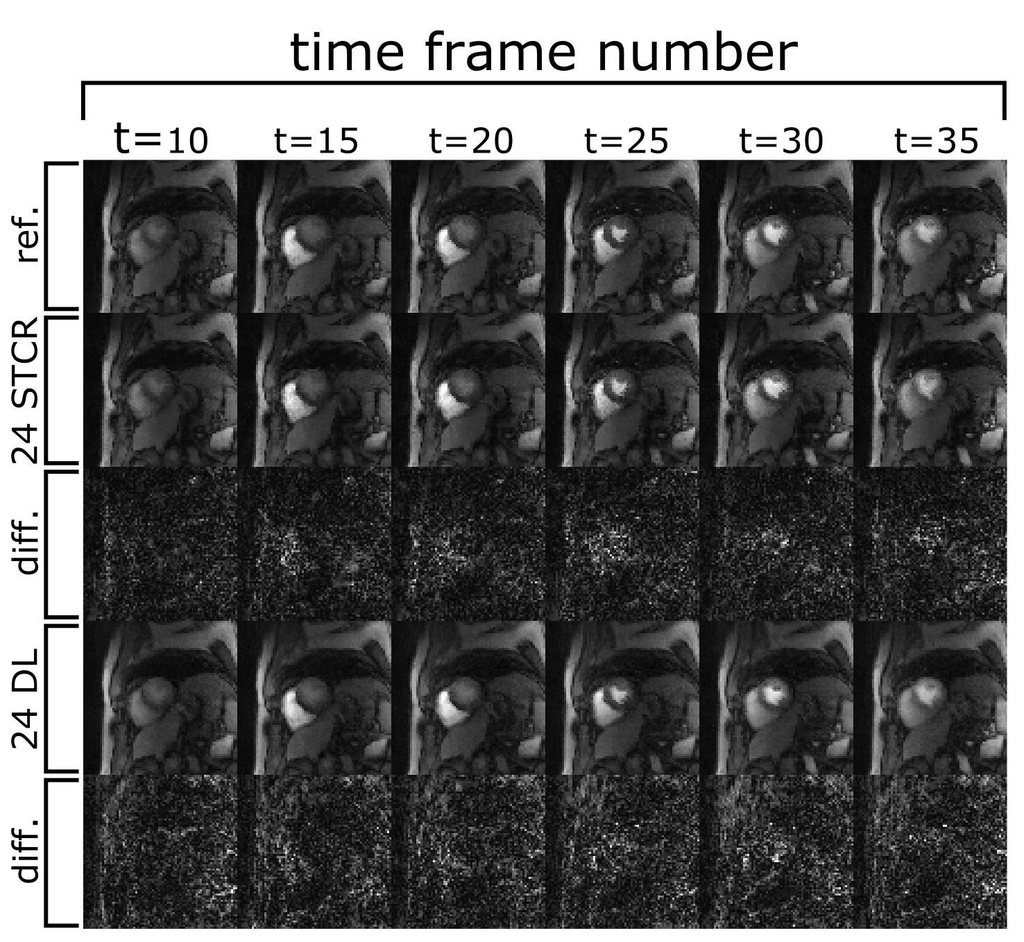
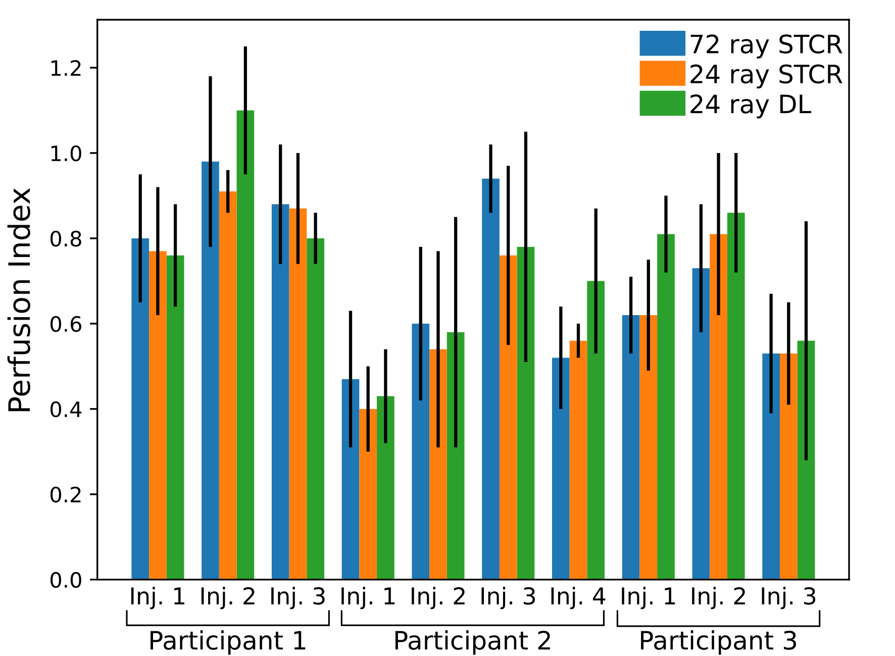
Fig. 2 shows example output images from the fully sampled reference and the undersampled 24 ray STCR and deep learning reconstructions. In the difference images between the 24 ray deep learning images and the reference, anatomical structures do not appear to be present, particularly in comparison with the undersampled STCR case. Looking at the contrast time curves in the blood pool in Fig. 3, the contrast in the images generated by the deep learning approach match with the reference closely. Additionally, the entire reconstruction process (from raw k-space data to final image) took 12-16 seconds using the deep learning methods. By contrast, the iterative approach took 3-4 minutes based on the number of frames and slices.

Fig. 4 shows the mean calculated perfusion index for each of the contrast injections for each of the test participants. These trends suggest that the deviations from the reference for the deep learning images are in line with what we see with established iterative reconstruction techniques.

Discussion and Conclusion

The results presented here show that a deep learning approach can give comparable results to images generated by iterative algorithms at a much lower computational cost. However, pushing beyond the results established here likely will require more training data as well as more exotic network architectures. Incorporating adversarial loss has been demonstrated to improve neural network performance in these reconstruction tasks. Additional validation is an important next step.

We have demonstrated a rapid method of generating high fidelity images from highly undersampled radial cardiac perfusion k-space datasets. This deep learning approach achieves considerably faster reconstruction times than iterative reconstruction methods.

Acknowledgements

No acknowledgement found.