Introduction

Cardiac MRI late gadolinium enhancement (LGE) imaging¹ based on inversion recovery sequences is well established to assess myocardial viability. The correct inversion time (TI) for nulling the healthy myocardium to optimize the contrast to scar tissue is key for good image quality. In current clinical practice, the selection is done by visual inspection of a TI scout acquisition which requires user expertise and interaction and is therefore prone to errors. Previously, the automated selection of TI using Deep Learning has been proposed; however, the proposed method does not provide a quantitative output². In this study, we investigate an automated TI selection and evaluate the feasibility by comparing it with annotations performed by two medical experts.

Methods

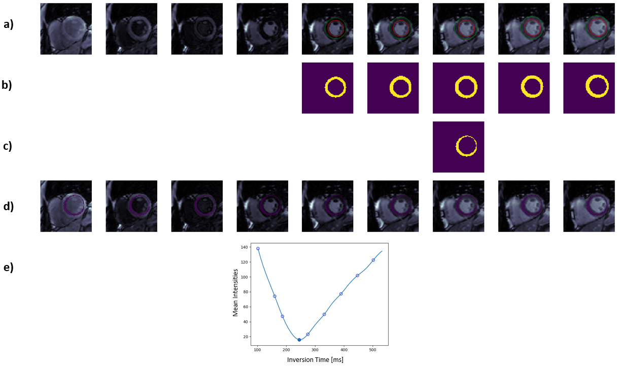
The proposed prototype system consists of four processing steps (Fig. 1). The system input is a TI scout sequence of a mid-ventricular short-axis slice, i.e. a time-resolved 2-D image series with varying contrast after an inversion pulse. The last frames of the TI scout have a similar appearance as CINE imaging when enough time has passed after the inversion pulse. In these frames, a deep-learning-based segmentation model previously trained on standard CINE images³ can be applied to segment the myocardium. After segmenting the myocardium at different positions of the cardiac cycle, we compute the intersection set of all myocardial segmentations. This allows us to identify pixel locations (those within the intersection set) that will likely also lie within the myocardium in frames where CINE segmentation cannot be performed due to different blood-myocardium contrast. Finally, the mean of the pixel intensities within the intersection set at each TI time point is calculated. The plot of the means over the time series represents the T1 recovery. The minimum point of the curve signifies the approximate nulling point (TI_null) of the myocardium with the lowest signal intensity.

Experiments

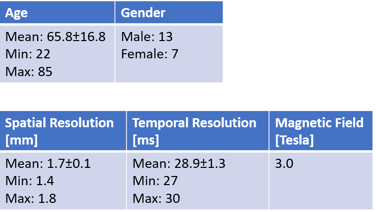
The proposed system is evaluated on short-axis TI scout acquisitions from 20 patients, acquired on 3T clinical MRI scanners (MAGNETOM Skyra, Siemens Healthcare, Erlangen, Germany). Details on patient population and data acquisition are provided in Fig. 2. The system has been validated by calculating the mean and the standard deviation of the absolute difference between TI_null and the optimal TI (TI_optimal) annotated by one observer (M.S., $$$>10$$$ years of cardiac MR experience). To compute intra- and inter-observer variability, a subset of 9 cases was additionally annotated twice on two different days by a second, independent observer (B.W., $$$>20$$$ years of cardiac MR experience). The system performance compared to each observer and the inter- and intra-observer statistics are assessed with Bland-Altman (BA) plots.

Results

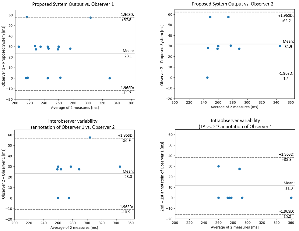
The mean difference of inversion times between observer 1 and the system was $$$23.1\pm17.7\,ms$$$ (n=20) and between observer 2 and the system $$$31.9\pm15.5\,ms$$$ (n=9). The BA plots are shown in Fig. 4. Comparing the differences between the system and observer 1, the timepoint selected by the algorithm was off by one frame from the annotation ($$$\sim30\,ms$$$) in $$$58\%$$$ of cases, same in $$$31\%$$$ of cases, and off by two frames ($$$\sim60\,ms$$$) in $$$11\%$$$ of cases. The comparison between the system and observer 2 shows that the timepoint selected by the algorithm was off by one frame ($$$\sim30\,ms$$$) in $$$70\%$$$ cases, two frames ($$$\sim60\,ms$$$) in $$$20\%$$$, and same in $$$10\%$$$ cases. The inter-observer variability plot shows that the result was off by one frame ($$$\sim30\,ms$$$) in $$$60\%$$$, the same in $$$20\%$$$ and by two frames in $$$10\%$$$. For the intra-observer variability, there is an exact match in $$$71.4\%$$$ of cases and $$$28.6\%$$$ varied by one frame.

Discussion

The automated TI_null selection was successfully performed in all datasets. The results demonstrate the ability of the algorithm to find the optimal TI for adequate myocardial nulling. However, this system relies on the performance of the segmentation network. The deviations between the TI_optimal chosen by each observer and the system are reasonable, as the optimal TI is selected after 1 or 2 frames ($$$30-60\,ms$$$) in most cases. The inter- and intraobserver variability reveals that choosing the optimal TI is a user-dependent task. Compared to previous work², where a time window with two classes (early, acceptable) is classified, this method provides an efficient process that outputs quantitative results and is more intuitive with its subsequent steps than the end-to-end neural network. Our method can be extended to orientations other than the short-axis by the use of a different segmentation network for those orientations. For the optimal TI, an adjustment might be needed; however, the first timepoint after TI_null can be a good starting point. As shown in the inter-observer statistics, the selection can vary by one or two frames. As stated in ⁴, it is better to choose the TI too late than too early. In none of the 20 cases have the TI_null been detected by the proposed algorithm at a later timepoint than the TIoptimal chosen by the observers. The proposed algorithm based on CINE segmentation can improve efficiency and reproducibility in clinical workflows.

Conclusion

Automated TI selection was successfully performed with high accuracy by the proposed system. Future work will focus on evaluating different cardiac orientations, the extension to 1.5T data as well as on clinical validation assessing the impact on LGE quantification.

Acknowledgements

No acknowledgement found.