2096
Flow Effects in AIF Measurements for Quantitative Myocardial Perfusion1Radiology and Imaging Sciences, University of Utah, Salt Lake City, UT, United States
Synopsis
We study the flow effects in AIF estimation for myocardial perfusion MRI. Simulations were performed and radially acquired datasets were retrospectively analyzed. We reconstruct images using
Introduction
Myocardial first-pass perfusion MRI can provide non-invasive, radiation-free diagnoses for coronary artery diseases. There is also increasing interest in getting quantitative myocardial blood flow (MBF) values from the first-pass perfusion images. Quantitative analysis requires an accurate estimation of the arterial input function (AIF). Popular methods for AIF estimations include the dual-bolus (1) or the dual-sequence (2) methods. However, the AIF can change across a cardiac cycle, and the diastolic AIF peak has been reported to be significantly higher than the systolic AIF peak (3); this may be caused by flow effects during the data acquisition. Here we study the flow effects with simulations and by retrospectively analyzing two types of human subjects datasets acquired with radial trajectories (4,5).Theory
A commonly used pulse sequence for quantitative myocardial perfusion is saturation recovery preparation followed by a FLASH readout. During a typical acquisition window of 70-150ms, ‘fresh’ blood flows into or out of the LV if not during the quiescent phase of diastole which is relatively short. The mixture of blood that has seen a different number of slice selective alpha pulses can result in a signal intensity that is higher than still blood, giving a higher AIF estimation.Radial trajectories go through the k-space center at every ray, such that each ray reflects the image contrast at that temporal point. We reconstructed radially acquired k-space data using a different number of rays starting from the first ray after each SR pulse and estimated AIF from each reconstruction. The AIFs estimated from different reconstructions should reflect different flow effects, with increasing flow effects in longer acquisition window.
Methods
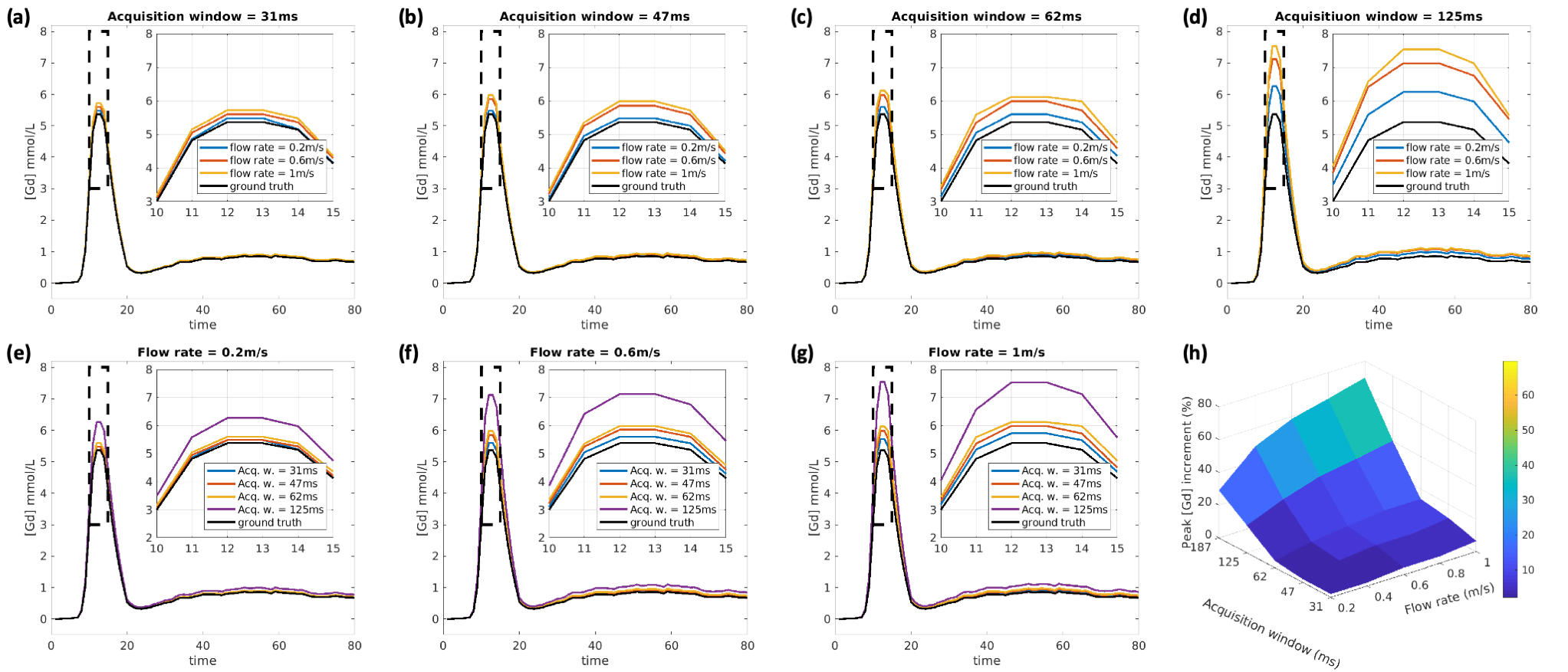
SimulationsAn in-vivo measured AIF [Gd] curve (acquisition window 47ms) was used in Bloch simulations as the ground truth. Different acquisition windows (31,47,62,125 and 187ms) combined with different constant flow rates (0.2,0.4,0.6,0.8 and 1m/s) were simulated. We chose TR=2.6ms, SRT=10ms, flip angle (FA)=14°.
Saturation recovery 72-ray datasets
Eleven patients with 46 injections (25 at stress) were acquired with TR/TE=2.6/1.1ms, SRT=10ms, FA=14°, 72 rays/frame, 2-4 short-axis slices per injection on a 3T scanner (5). Proton density (PD) weighted images were also acquired for each patient.
Continuous radial SMS (cSMS) datasets
Ten injections (3 were stress) from 7 patients acquired with TR/TE=2.5/1.2ms, SRT=10ms, and FA=14° were analyzed. Three slices were acquired simultaneously with a CAIPIRINHA phase modulation (6,7). A saturation pulse was applied after each ECG trigger, and radial data acquisition continued until the next trigger (4).
AIF estimation
For each dataset, five sets of AIFs were estimated from images reconstructed using different number of rays per time frame. We chose 12,18,24,48 and 72 rays/frame, correspond to acquisition windows of 31, 47, 62, 125 and 187ms.
For each injection, a region of interest (ROI) was drawn in the LV and the pixel intensities in the ROI were averaged to be the signal intensity (SI) curve. A look-up-table generated from Bloch simulations was used to convert measured SI curves (normalized by PD images) into gadolinium concentration curves.
Results
SimulationFigure 1 shows the simulation results with different acquisition windows combined with different flow rates. The flow effects can increase the AIF estimation up to 70% with the highest flowrate and the longest acquisition window. However, with a short acquisition window (31 or 47ms), the overestimation was less than 11%.
In-vivo measurements
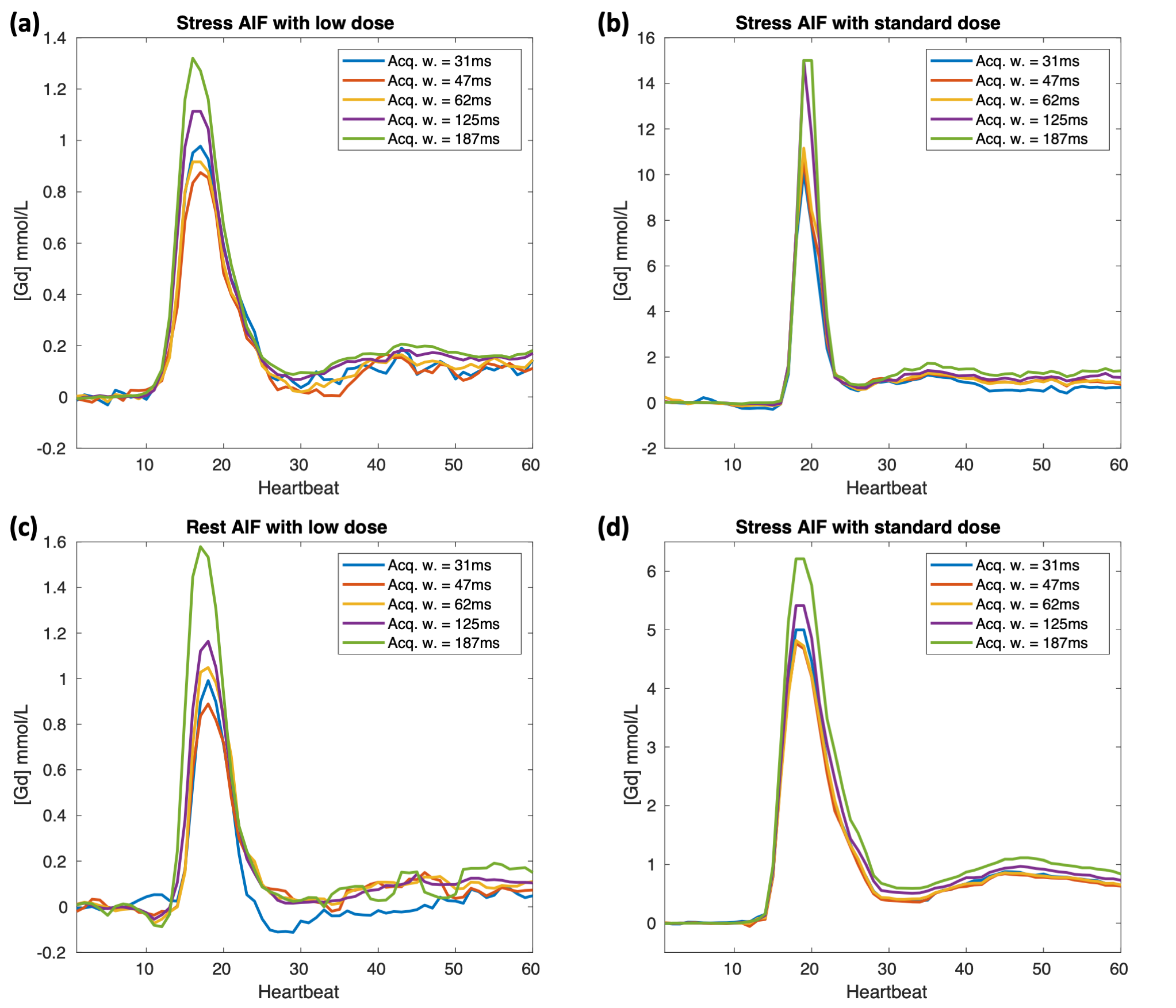
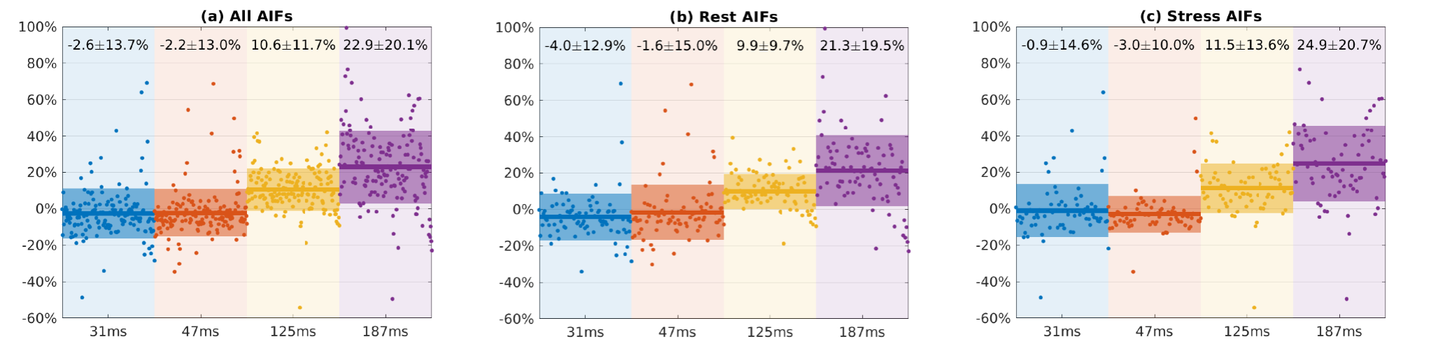
Figure 2 shows four typical AIFs at different injection doses and different physiological states (stress or rest), where the longer acquisition led to a higher AIF. Figure 3 summarizes all the results, including 148 sets of AIFs (each set has 5 AIFs with different acquisition windows) from 56 injections (2-4 slices per injection) of 18 patients. We used the 62ms AIF as a reference to calculate the percentage difference:
$$\mathrm{Percentage\quad Difference}=\frac{[\mathrm{Gd}]_{\mathrm{peak}}-[\mathrm{Gd}]_{\mathrm{peak}}^{\mathrm{ref}}}{[\mathrm{Gd}]_{\mathrm{peak}}^{\mathrm{ref}}},$$
where $$$[\mathrm{Gd}]_{\mathrm{peak}}$$$ is averaged 3 highest $$$[\mathrm{Gd}]$$$ values in each AIF curve. The $$$[\mathrm{Gd}]_{\mathrm{peak}}$$$ shows a small trend of increase (<5%) at low acquisition windows (31-62ms). With a longer acquisition window, the increase is significant, at 10.6% for 125ms and 22.9% for 187ms. The increase does not have a significant difference between stress and rest.
Discussion and Conclusion
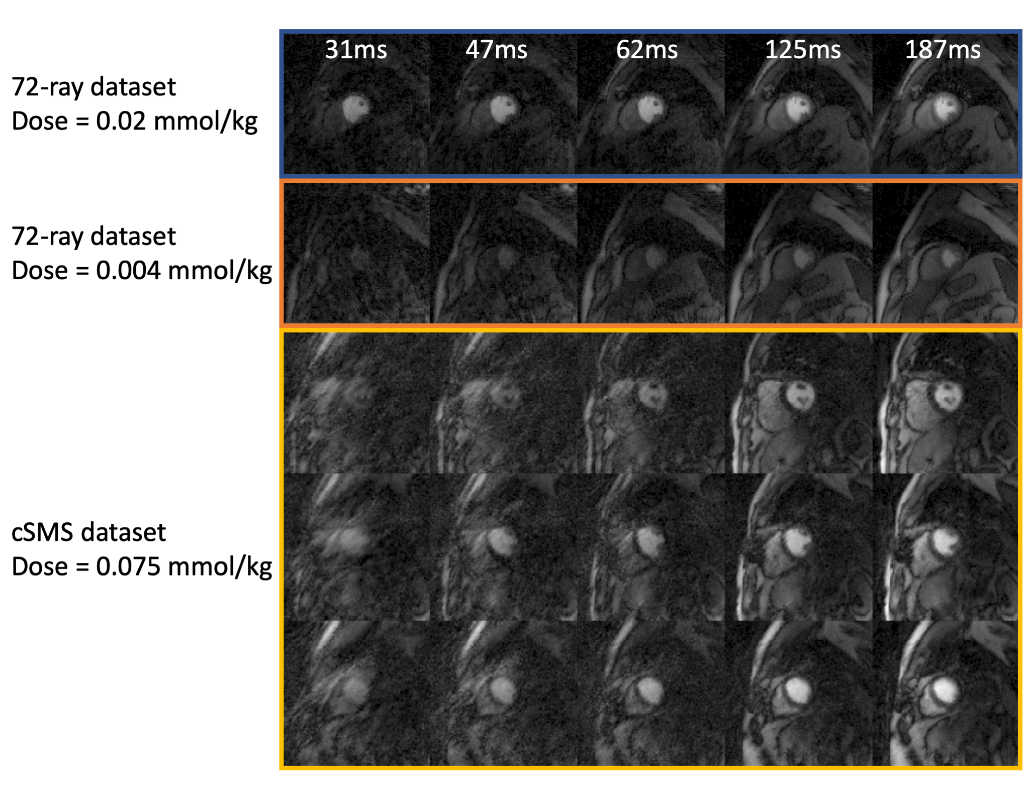
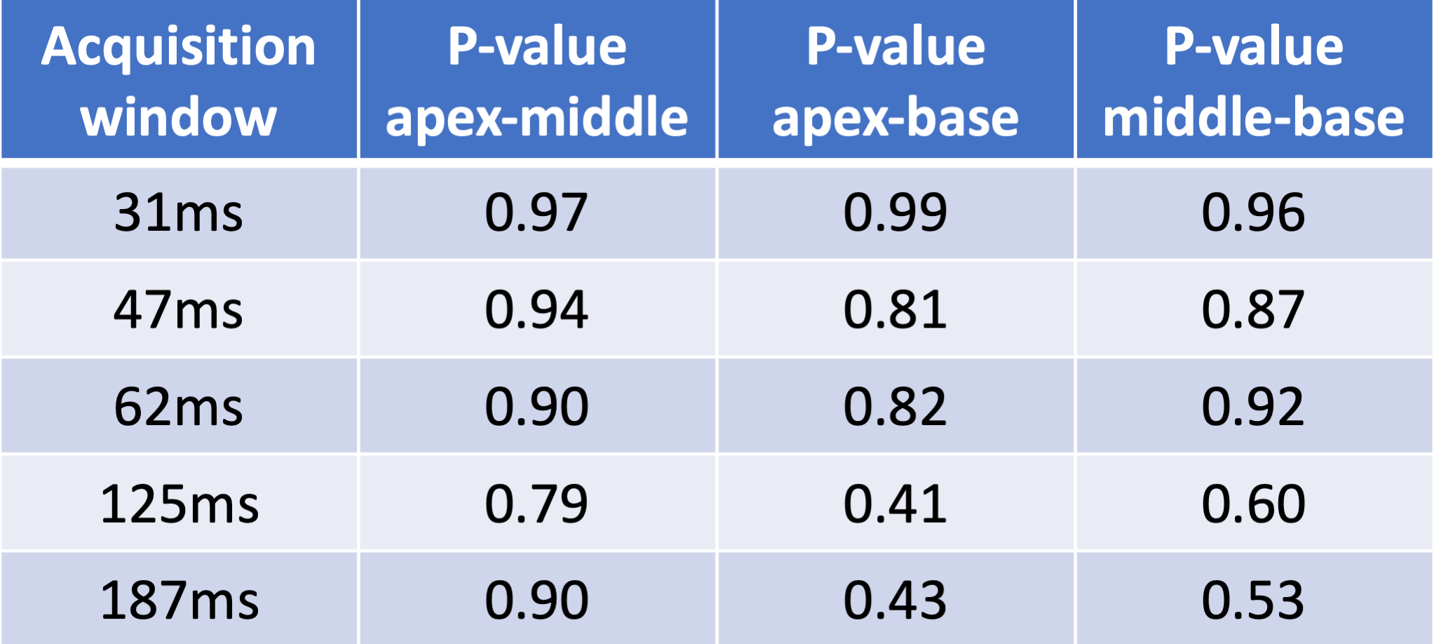
The study was done on radially acquired datasets. With Cartesian or spiral trajectories, the flow effects are different. With a centric Cartesian readout, arguably the flow effects can be minimal, however the image may suffer from an inherent high-pass filtering (8). With a linear Cartesian readout, the flow effects come from the k-space center readout, and may be similar with radial trajectories that average flow effects from all readouts. The 12-ray and 18-ray reconstructions suffer from artifacts as shown in Figure 4, but they may still provide useful AIF estimations, since averaging pixels in LV increase the signal-to-noise level. We also studied AIF difference across the apex, middle and base LV from 42 injections that have at least 3 slices and show the results in Figure 5.The AIF estimation form the LV for quantitative myocardial perfusion is higher with an increased acquisition window; this is likely related to flow effects. A short acquisition window below or around 62ms and/or acquisition during a period of minimal LV blood flow is desired to acquire AIF with little flow effects when using a radial trajectory.
Acknowledgements
No acknowledgement found.References
1. Christian TF, Aletras AH, Arai AE. Estimation of absolute myocardial blood flow during first-pass MR perfusion imaging using a dual-bolus injection technique: comparison to single-bolus injection method. J Magn Reson Imaging 2008;27(6):1271-1277.
2. Gatehouse PD, Elkington AG, Ablitt NA, Yang GZ, Pennell DJ, Firmin DN. Accurate assessment of the arterial input function during high-dose myocardial perfusion cardiovascular magnetic resonance. J Magn Reson Imaging 2004;20(1):39-45.
3. Radjenovic A, Biglands JD, Larghat A, Ridgway JP, Ball SG, Greenwood JP, Jerosch-Herold M, Plein S. Estimates of systolic and diastolic myocardial blood flow by dynamic contrast-enhanced MRI. Magn Reson Med 2010;64(6):1696-1703.
4. DiBella E, Likhite D, Adluru G, Welsh C, Wilson B. A New Hybrid Approach for Quantitative Multi-Slice Myocardial DCE Perfusion. 2016; Singapore. In the proceddings of ISMRM 2016 annual meeting. p 463.
5. Kim TH, Pack NA, Chen L, DiBella EV. Quantification of myocardial perfusion using CMR with a radial data acquisition: comparison with a dual-bolus method. J Cardiovasc Magn Reson 2010;12:45.
6. Wang H, Adluru G, Chen L, Kholmovski EG, Bangerter NK, DiBella EV. Radial simultaneous multi-slice CAIPI for ungated myocardial perfusion. Magn Reson Imaging 2016;34(9):1329-1336.
7. Yutzy SR, Seiberlich N, Duerk JL, Griswold MA. Improvements in multislice parallel imaging using radial CAIPIRINHA. Magn Reson Med 2011;65(6):1630-1637.
8. Kellman P, Hansen MS, Nielles-Vallespin S, Nickander J, Themudo R, Ugander M, Xue H. Myocardial perfusion cardiovascular magnetic resonance: optimized dual sequence and reconstruction for quantification. J Cardiovasc Magn Reson 2017;19(1):43.
Figures