Introduction

While rapid k-space coverage techniques such as EPI and Spiral have become popular tools in MR, little has been done to address the image blurring caused by T2* signal decay during the readout. This is particularly troublesome in applications with long readouts and low T2* values, such as, but not exclusively, diffusion tensor cardiovascular magnetic resonance (DT-CMR). We previously implemented a method that corrects spiral DT-CMR images assuming a constant myocardial T2* ¹. Here, we extend this work to account for the known spatial variations in T2* within the myocardium and we also show a novel stimulated echo-based spiral T2* mapping method with B0 correction. The methods are first tested in simulations and then in-vivo data.

Methods

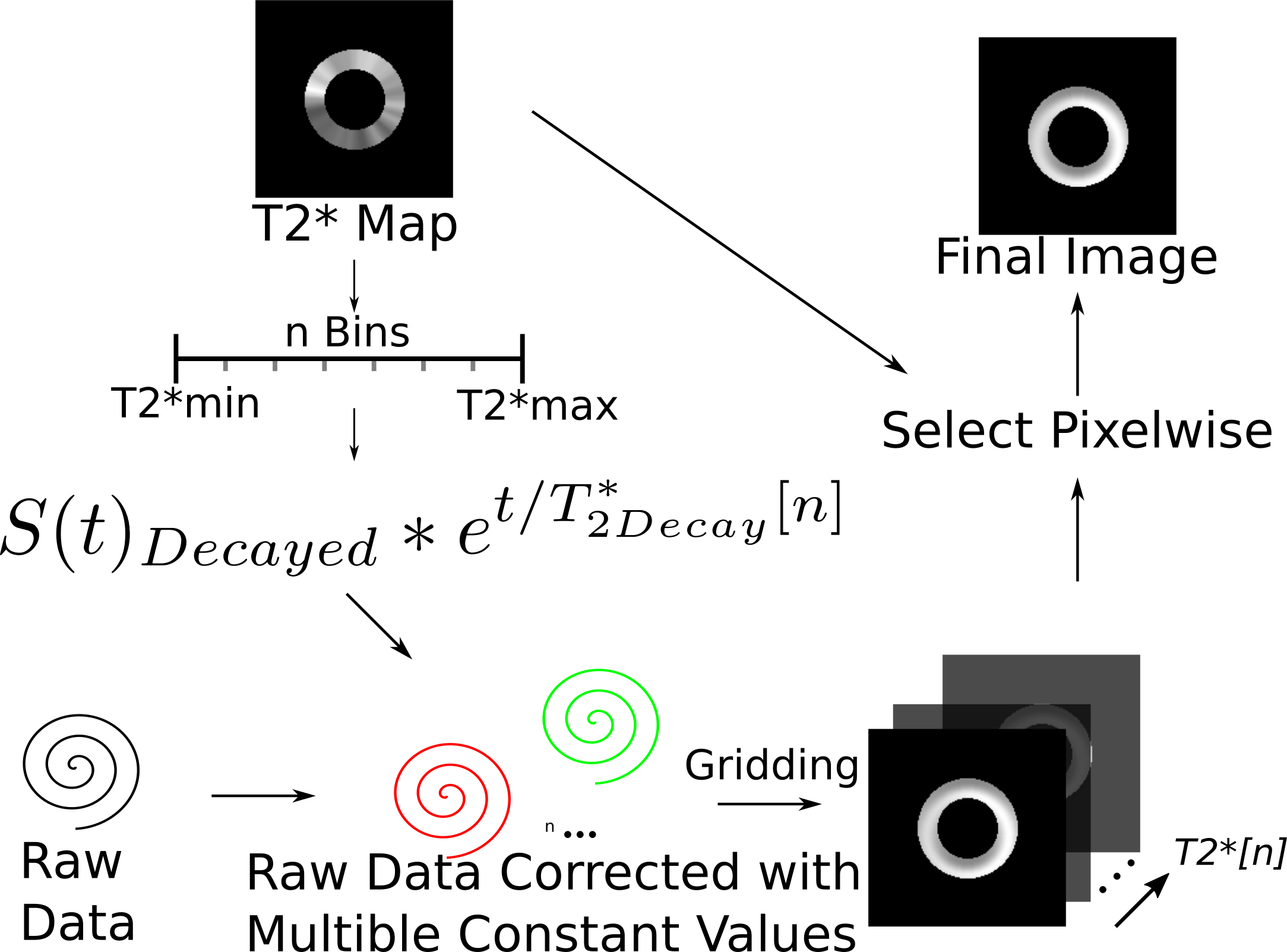
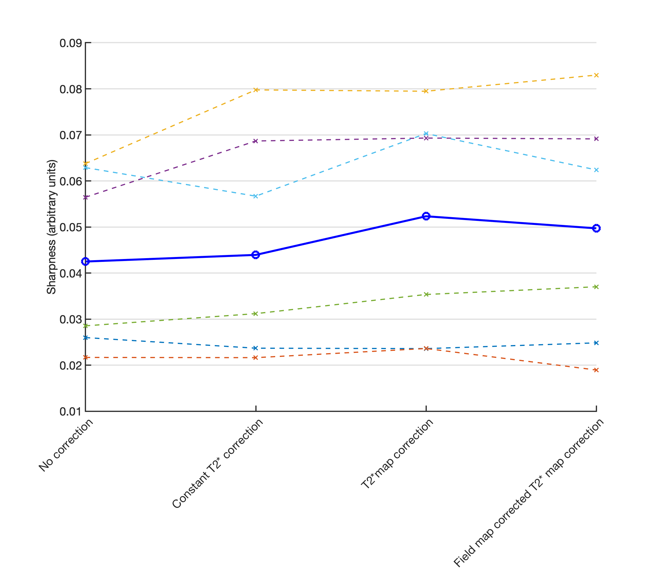
Spatially uniform and varying T2* corrections were initially evaluated using a synthetic single-short axis slice cardiac DT-CMR dataset (b-values 150smm^-2 and 600smm^-2, 6 directions, mean b0 SNR=27). Simulated T2* varied linearly around the circumference and a 2mm thick region of simulated pathology was included, circumferentially spiralling from epi to endocardium. Spiral cardiac DT-CMR dataset was acquired in 6 healthy volunteers (age 27-64, 2 female,4 male) for a short axis slice. T2* mapping data was acquired with a Stimulated Echo Acquisition Mode (STEAM) prepared method with a spiral trajectory. The T2* mapping sequence was acquired in one breath hold, of 22 cardiac cycles. Two cardiac cycles were required for each stimulated echo and one stimulated echo was used for the coil sensitivity maps, two for the field (B0) maps and eight for the T2* mapping data. T2* mapping used 8 ∆TE (time from the stimulated echo to the beginning of the spiral) linearly varying from 0 ms to 16 ms. Spiral STEAM DT-CMR data were then acquired at b=150smm^-2 with 6 directions. Both T2* mapping data and DT-CMR were acquired with a reduced field of view using in-plane slice selective RF pulse, 2.8x2.8x8mm³ acquired spatial resolution, 90x90mm² spiral readout field of view, spiral duration 14.9ms. All data were acquired on a Vida XT 3T system (Siemens Healthineers Erlangen). T2* maps were calculated before and after a frequency segmented B0 correction² of the raw T2* images. Based on the frequency segmented reconstruction² the novel spatially varying T2* correction is shown in Figure 1. Reconstructed with 40 different uniform T2* corrections a set of images was created by standard gridding operations. The final image was then obtained by pixelwise selection of the data corresponding to the T2* value in the T2* map. The data were reconstructed using a custom Gadgetron³ based online reconstruction, that reconstructed in 16s (spatially varying correction, Intel i9-7940X CPU, 32GB RAM). Image sharpness was assessed in a region of the left ventricular septal endocardial border using the edge sharpness fitting described previously⁴. Diffusion weighted images were compared without T2* correction, with uniform T2* correction (using mean myocardial T2*) and with spatially varying T2* correction both with and without off-resonance correction of the T2* data.

Results

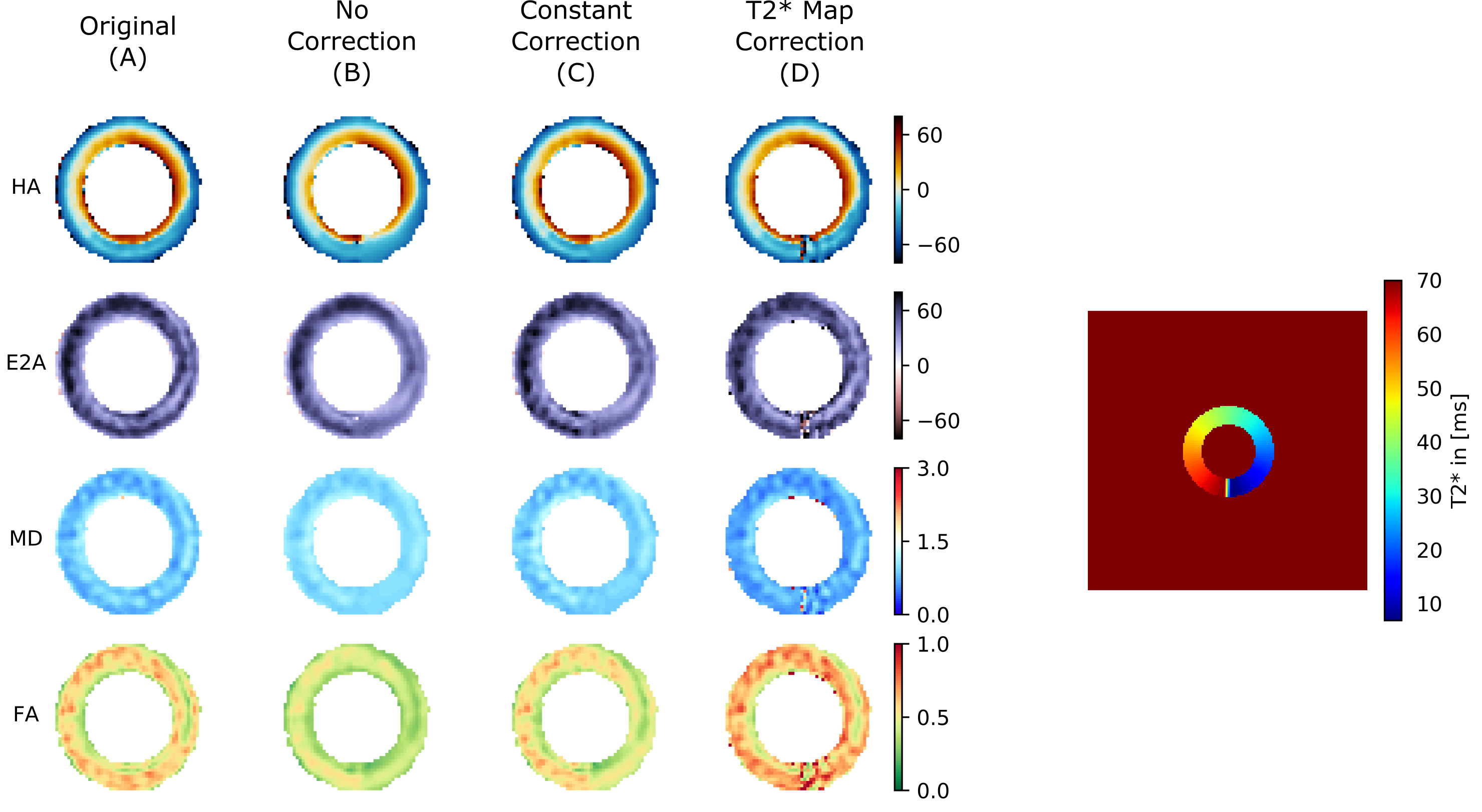
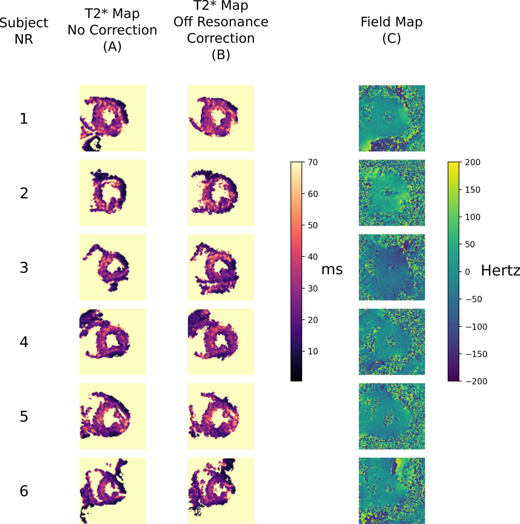
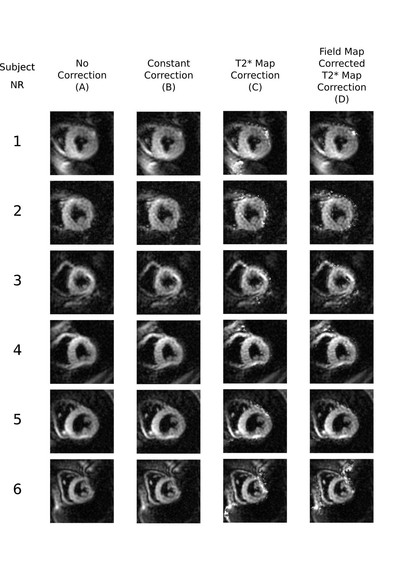
Figure 2 shows the DT-CMR maps from the simulations and the different corrections. While T2* related blurring in the region of simulated pathology is improved in the constant correction it is lowest when using the spatially varying correction. The T2* maps and associated B0 maps for each subject are shown in Figure 3. T2* maps are shown with and without off-resonance correction. These T2* maps were then used to correct the results shown in Figure 4. Spatially varying T2* correction results in visually sharper images at the expense of some spurious pixel values in the image background and myocardial borders. Figure 5 shows the sharpness measures for each of the T2* correction methods. The spatially varying T2* correction without off-resonance correction of the T2* maps yield the highest sharpness values.

Discussion

We have shown that it is possible with our novel method to correct for spatially varying T2* related blurring in spiral images. The images corrected with our novel method demonstrate improvement in sharpness measures over the images corrected with a constant T2* value and uncorrected images. However, visually there are errors in some pixels after correction, particularly at the myocardial borders. This noise enhancement is due to low measured T2* values and background noise and might be reduced through regularization methods, such as ⁵, applied to the T2* map calculation. We did not apply off-resonance correction to the imaging data, as joint T2* and B0 correction is computationally challenging but is expected to improve our image quality. This improvement in sharpness will be important as spatial resolution is improved and applied in challenging anatomy and patient cohorts, including the right ventricle. While we have chosen to demonstrate the improvement in sharpness in DT-CMR data, the T2* correction method may be of use in other applications using spiral trajectories or other long readouts.

Conclusion

Non uniform T2* causes spatially varying image blurring in methods with long readouts such as spiral DTCMR. For the first time, we show that this blurring can be corrected based on T2* maps.

References

1. Gorodezky, M, Ferreira, PF, Nielles‐Vallespin, S, et al. High resolution in‐vivo DT‐CMR using an interleaved variable density spiral STEAM sequence. Magn Reson Med. 2019; 81: 1580– 1594. https://doi.org/10.1002/mrm.27504
2. Noll, D. C., Pauly, J. M., Meyer, C. H., Nishimura, D. G. and Macovskj, A. (1992), Deblurring for non‐2D fourier transform magnetic resonance imaging. Magn. Reson. Med., 25: 319-333. doi:10.1002/mrm.1910250210
3. Hansen, M. S. and Sørensen, T. S. (2013), Gadgetron: An open source framework for medical image reconstruction. Magn Reson Med, 69: 1768-1776. doi:10.1002/mrm.24389
4. Ahmad, R. , Ding, Y. and Simonetti, O. P. (2015), Edge sharpness assessment by parametric modeling: Application to magnetic resonance imaging. Concepts Magn. Reson., 44: 138-149. doi:10.1002/cmr.a.21339
5. A. K. Funai, J. A. Fessler, D. T. B. Yeo, V. T. Olafsson and D. C. Noll, "Regularized Field Map Estimation in MRI," in IEEE Transactions on Medical Imaging, vol. 27, no. 10, pp. 1484-1494, Oct. 2008. doi: 10.1109/TMI.2008.923956