2003
The impact of B1+ inhomogeneities on automatic hippocampal morphometry using 7T MRI
Roy AM Haast1, Jonathan C Lau1,2, Dimo Ivanov3, Kamil Uludag4,5, and Ali R Khan1,6
1Robarts Research Institute, Western University, London, ON, Canada, 2Department of Clinical Neurological Sciences, Division of Neurosurgery, Western University, London, ON, Canada, 3Department of Cognitive Neuroscience, Maastricht University, Maastricht, Netherlands, 4Institute for Basic Science, Center for Neuroscience Imaging Research, Department of Biomedical Engineering, Sungkyunkwan University, Suwon, Republic of Korea, 5University Health Network, Toronto, ON, Canada, 6Department of Medical Biophysics, Schulich School of Medicine and Dentistry, Western University, London, ON, Canada
1Robarts Research Institute, Western University, London, ON, Canada, 2Department of Clinical Neurological Sciences, Division of Neurosurgery, Western University, London, ON, Canada, 3Department of Cognitive Neuroscience, Maastricht University, Maastricht, Netherlands, 4Institute for Basic Science, Center for Neuroscience Imaging Research, Department of Biomedical Engineering, Sungkyunkwan University, Suwon, Republic of Korea, 5University Health Network, Toronto, ON, Canada, 6Department of Medical Biophysics, Schulich School of Medicine and Dentistry, Western University, London, ON, Canada
Synopsis
We examined the effect of B1+ inhomogeneities in 7T MP2RAGE data on hippocampal morphometry using volume- and surface-based evaluation methods. As for the cortex, significant variability in hippocampal and subcortical segmentation outputs are observed between original and corrected MP2RAGE data, especially near GM-CSF boundaries. Importantly, results of data acquired at two sites, using different MR hardware and sequence setups (B1+-sensitive vs insensitive), become more comparable after B1+ correction. These data emphasize the dependency of segmentation performances on anatomical image quality, and stresses the need for careful consideration of sequence parameters when setting up imaging protocols.
Introduction
Ultra-high field (≥ 7T) MRI suffers from transmit and receive B1-related image inhomogeneities which can hamper the correct classification of tissue types. Our initial report showed that residual B1+ (transmit) inhomogeneities in the T1-weighted and quantitative T1 images, acquired using the MP2RAGE sequence at 7T, lead to biases in cortical thickness measurements[1]. We observed strong changes in T1 and thickness in temporal and frontal cortices, especially, when data were corrected for these B1+-related image inhomogeneities. However, the effect on subcortical morphometry has not been studied so far. As such, the current analyses aim to expand our previous work by studying the effects on subcortical and hippocampal segmentation, in particular. Moreover, as these changes heavily rely on the B1+ sensitivity of the specific MR hardware (e.g., single vs. parallel transmit) and MP2RAGE sequence setups[2], we expect these biases to differ between acquisition sites. Therefore, the current work replicates the initial study (at Maastricht University, Maastricht, Netherlands) using an additional, independent dataset acquired at Western University (London, Ontario, Canada), to compare the effect of B1+ sensitivity on the observed (sub)cortical T1 and thickness/volume biases.Methods
Acquisition: Whole-brain MP2RAGE[2] and Sa2RAGE[3] data were acquired in Maastricht (n=16) and London (n=28) using a 7T MRI scanner (Siemens Healthineers, Erlangen, Germany). Acquisition hardware and sequences parameters for each dataset are specified in Figures 1A and B, respectively. Note, for the London dataset sequence parameters were chosen to render it minimally sensitive for B1+ differences (see Figure 1C).Analyses: MP2RAGE T1w and quantitative T1 maps were corrected for B1+ inhomogeneities[2]. The original and corrected T1w data were then used for longitudinal processing within FreeSurfer (v6.0)[4]. B1+ effects on subcortical and hippocampal morphometry were evaluated using volume- (i.e., total volume [mm3], Dice overlap [%] and Hausdorff distance scores), and surface-based (i.e., large deformation diffeomorphic metric mapping [LDDMM][5]) methods using openly available image processing scripts developed in-house (https://github.com/khanlab/surfmorph). Moreover, we computed the gradient magnitude for FreeSurfers' WM normalized output to relate segmentation changes to changes in the underlying anatomical contrast at the structures' boundaries. Finally, average quantitative cortical T1 and thickness before and after B1+ correction were compared by projection onto the reconstructed cortical surfaces.
Statistical analysis: we used mixed model analysis of variance (ANOVA) to test for differences between original and corrected subcortical structures’ volumes, segmentation evaluation metrics as well as potential differences between hemispheres, acquisition sites and/or interactions between these. Inter-site differences in surface displacement, and changes in gradient magnitude were explored using the SurfStat toolbox (http://www.math.mcgill.ca/keith/surfstat/) for Matlab (R2018b, The Mathworks, Natick, MA, USA). Vertex-wise one-sided T-tests were used for identification of vertices characterized by larger absolute surface displacement, and gradient change for the Maastricht dataset after correction for multiple comparisons using random field theory for non-isotropic images.
Results
Visual inspection of the reconstructed surface meshes (Figure 1A) show local differences in hippocampal surface placement between original and corrected labels. Compared to the Maastricht data, label overlap is significantly larger (F(1,42)=266.41, p<0.001), and distances between boundaries smaller (F(1,42)=23.20, p<0.001) for the London data (Figure 1B). As a result, slightly larger changes are observed for the Maastricht data considering hippocampal volume, especially after taking into account differences between left and right hemispheres, characterized by a significant interaction effect (F(1,42)=18.83, p<0.001, Figure 1C/D/E).LDDMM allows more precise quantification (Figure 3B) and localization (Figure 3A, single subject, and C, per group) of changes in hippocampal boundary placement. The white-dotted pattern indicates areas where changes are significantly stronger for the Maastricht dataset (p<0.05). Surface placement changed more strongly closer to the tail and head regions, apparent by the deep-blue and red coloring, corresponding to in-/outward placement in the original data, respectively.
Figure 4A highlights the extent of gradient magnitude changes. Differences between acquisition sites are spatially widespread, indicated by the white-dotted pattern (p<0.05), but tend to localize more towards the lateral (i.e. ‘outside’) and longitudinal (i.e.. head and tail) extents (Figure 4B). Especially the tail region seems to be affected most considering the overlap (purple patches in C) of both significant surface displacement (red) and gradient (blue) changes. Gradient magnitude changes more strongly closer to CSF (Figure 5A/B, cyan arrow/dots) and arteries (red arrow/mesh). While there is no direct relationship between surface displacement and distance to CSF (dashed orange line), gradient changes tend to become less strong, and less variable across subjects, moving away from the CSF (green line).
Discussion
Removal of residual B1+-related inhomogeneities in MP2RAGE data leads to changes in hippocampal, as well as subcortical (not shown here), morphometry. In general, changes in inter-tissue contrast due to the B1+ correction[2], although at GM-CSF interfaces predominantly, lead to variability in the segmentation accuracy (1) along the structures border, (2) between hemispheres, as well as (3) across subjects. We confirm that these effects strongly depend on the B1+ sensitivity of the MP2RAGE sequence setup, based on the large difference between the acquisition sites. Although we only focused on hippocampal morphometry here, our data shows that B1+ correction leads to increased inter-site comparability considering quantitative (sub)cortical T1, thickness and volume. These findings are especially important to take into account when setting up imaging protocols for analyzing and interpreting patient-based volumetric measurements.Acknowledgements
The author Roy AM Haast is supported by the BrainsCAN postdoctoral fellowship for this work. This research is enabled in part by support provided by Compute Canada (www.computecanada.ca).References
[1] Haast et al. (2018) Hum Brain Mapp. (6):2412-2425. [2] Marques & Gruetter (2013) PLoS One. 8(7):e69294. [3] Eggenschwiler (2012) Magn Reson Med. (6):1609-19. [4] Dale et al. (1999) Neuroimage. (2):179-94. [5] Khan et al. (2019) Neuroimage Clin. 21:101597.Figures
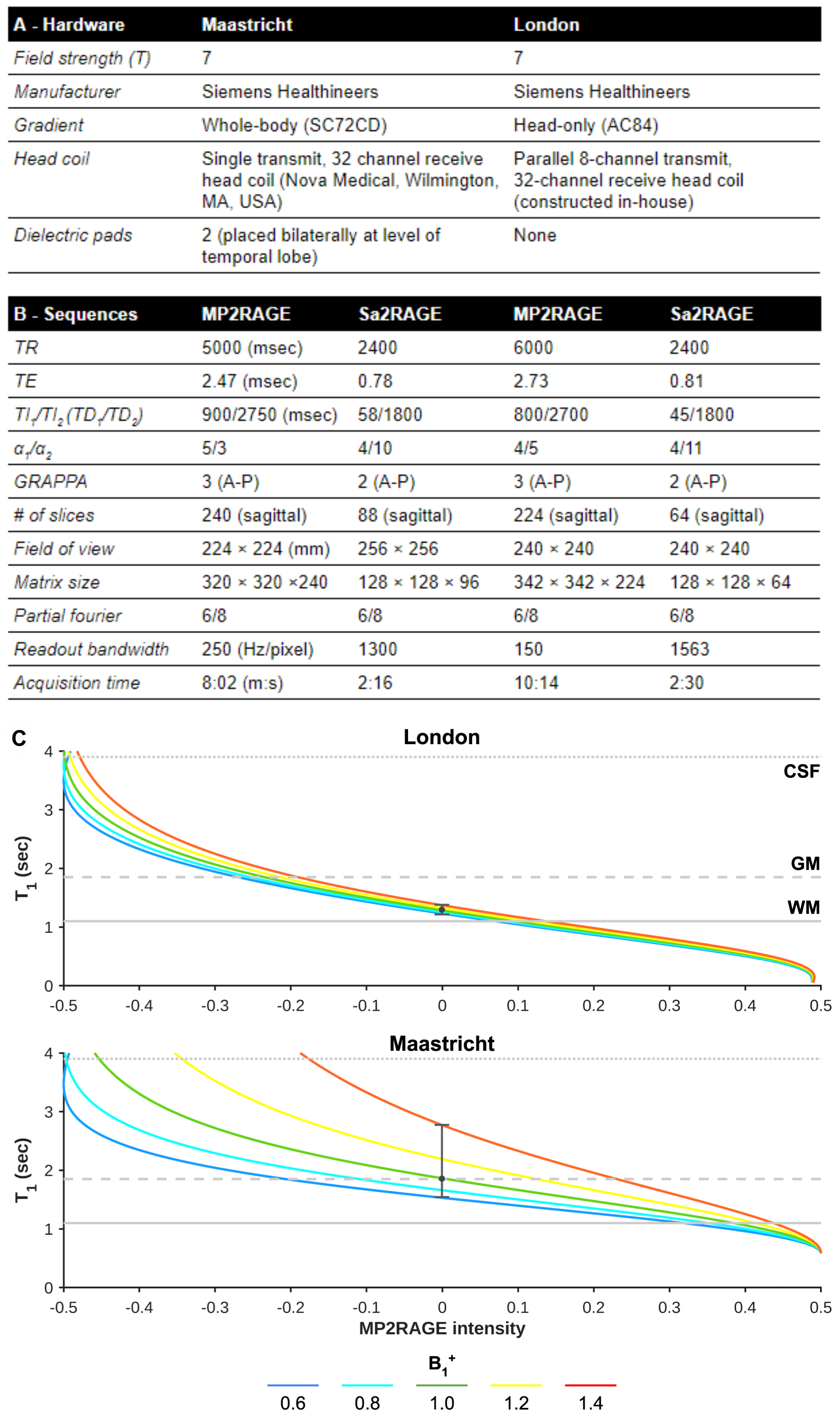
Figure 1 - (A) MRI scanner and (B) sequence set ups, specified per dataset. (C) B1+ dependency of the T1 map for a range of B1+ values (colored solid lines) for each acquisition site’s MP2RAGE protocol (top and bottom panel). Typical WM, GM, and CSF T1 values are indicated using the vertical lines.
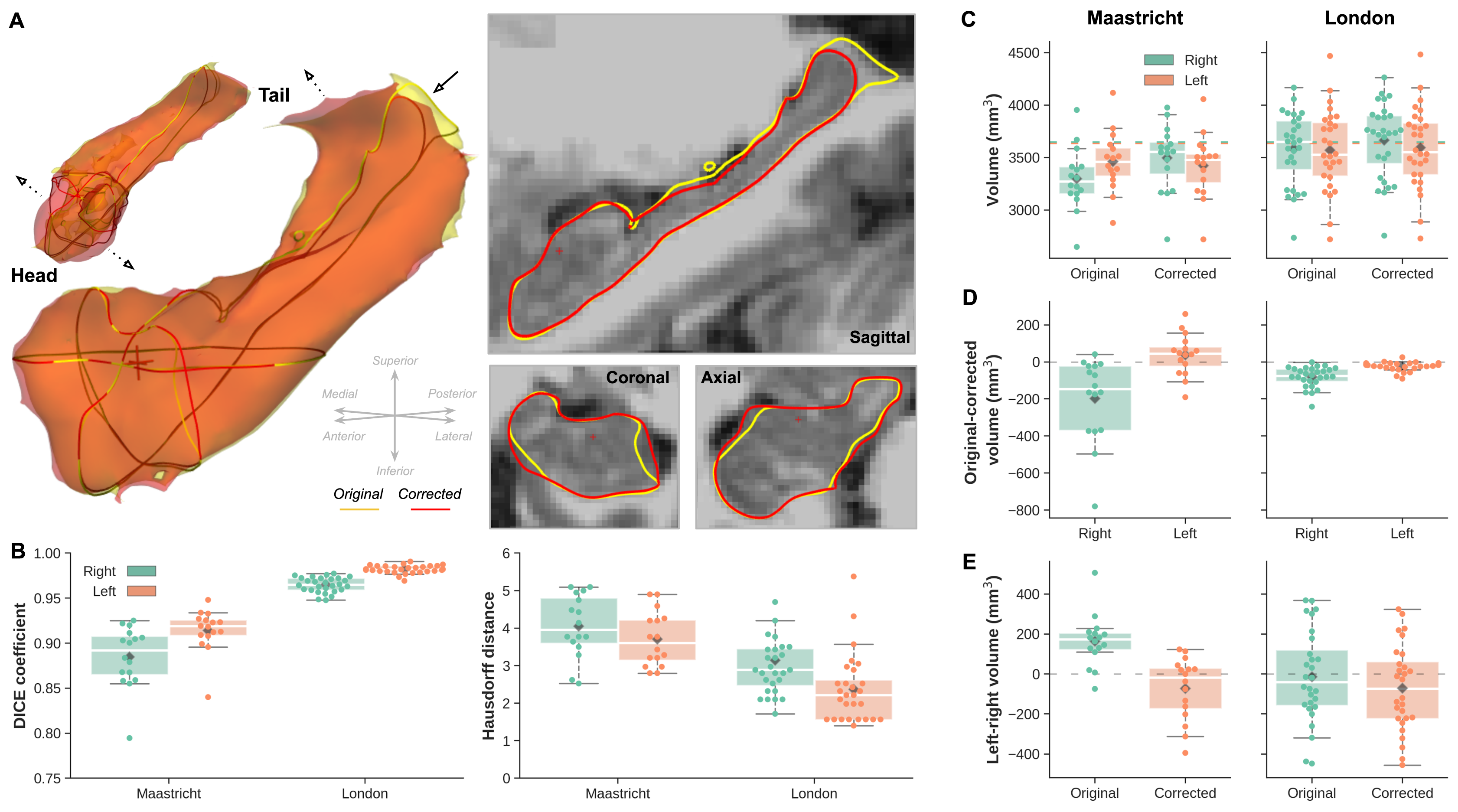
Figure 2 - (A) Single-subject example of left and right hemisphere hippocampal surfaces after processing the original (yellow) and corrected (red) MP2RAGE data. Sagittal, coronal and axial cross sections of the left hemisphere surface outlines are shown on the right. (B) Box plots showing distribution of original vs. corrected hippocampal Dice coefficient (left) and Hausdorff distance (right) for both acquisition sites (x-axis), and right (green) and left (orange) hemispheres. (C/D/E) Volume comparison between acquisition sites, original and corrected data and hemispheres.

Figure 3 - (A) Single-subject example from the Maastricht dataset showing the color-coded hippocampal surface displacement between original and corrected data. (B) Distribution plots showing the averaged hippocampal surface displacement for the Maastricht (left) and London (right) datasets. Inset figures show corresponding sagittal cross section of the left hemisphere hippocampus. (C) Surface representation of average displacement for both acquisition sites shown from an anterior (top) and posterior (bottom) perspective.

Figure 4 - For each acquisition site (left and right column): (A) Distribution plots showing the averaged change in gradient magnitude after B1+ correction at the original hippocampal boundaries. (B) Surface representation of the average change in gradient for both acquisition sites shown from an anterior perspective. (C) Overlap (in purple) of statistically different vertices based on surface displacement (red) and change in gradient (blue).
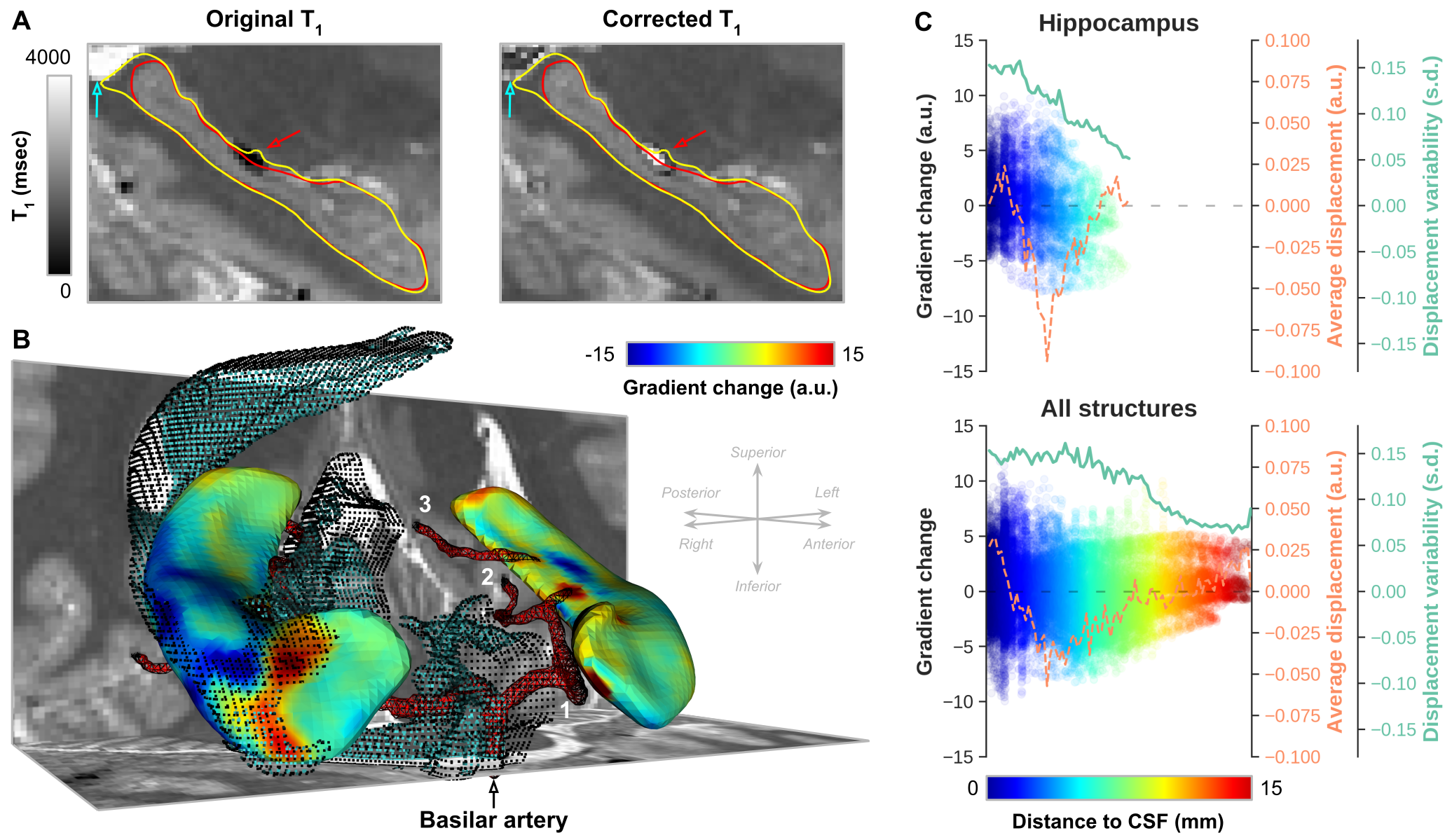
Figure 5 - (A) Single-subject example from the Maastricht dataset showing the original and corrected T1 (msec) maps and hippocampal segmentations from Figure 2A. (B) Surface representation of the changes in gradient magnitude along hippocampal boundaries (yellow contours in A), neighboring CSF and major arteries. (C) Vertex-wise gradient magnitude changes, across subjects average displacement (orange line) and standard deviation (green) as a function of the shortest distance to CSF (color-coded) for hippocampus only (top) and all structures together (bottom).