Introduction

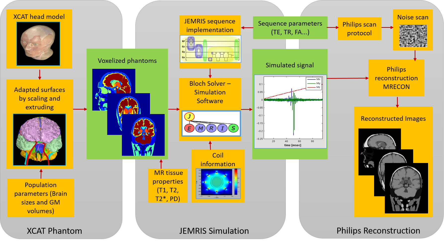
To make simulated MRI more realistic, a number of factors need to take into account. Including the use of finely structured phantoms with comprehensive tissue classes, true tissue properties, realistic simulation and realistic reconstruction. All these elements are integrated in our simulation pipeline by making use of XCAT phantom¹, JEMRIS simulation software² and clinically used Philips MRI reconstruction pipeline. The images generated using this pipeline, came out to be more realistic. Furthermore, to fill the gap of not having large sets of MRI data to be used for training and validating medical imaging analysis algorithms, a first set of anatomically variable simulated brain MRI images was created across age and gender using this pipeline. In previous studies^3,4, only a limited number of brain sub-structures were simulated and no steps were taken to simulate full head and aging brain MRI. A greater number of simulated tissue classes and anatomical variability is required to test and optimize algorithms to segment respective tissues. Our simulations included comprehensive set of tissues, anatomical variability as well as pathology.

Methods

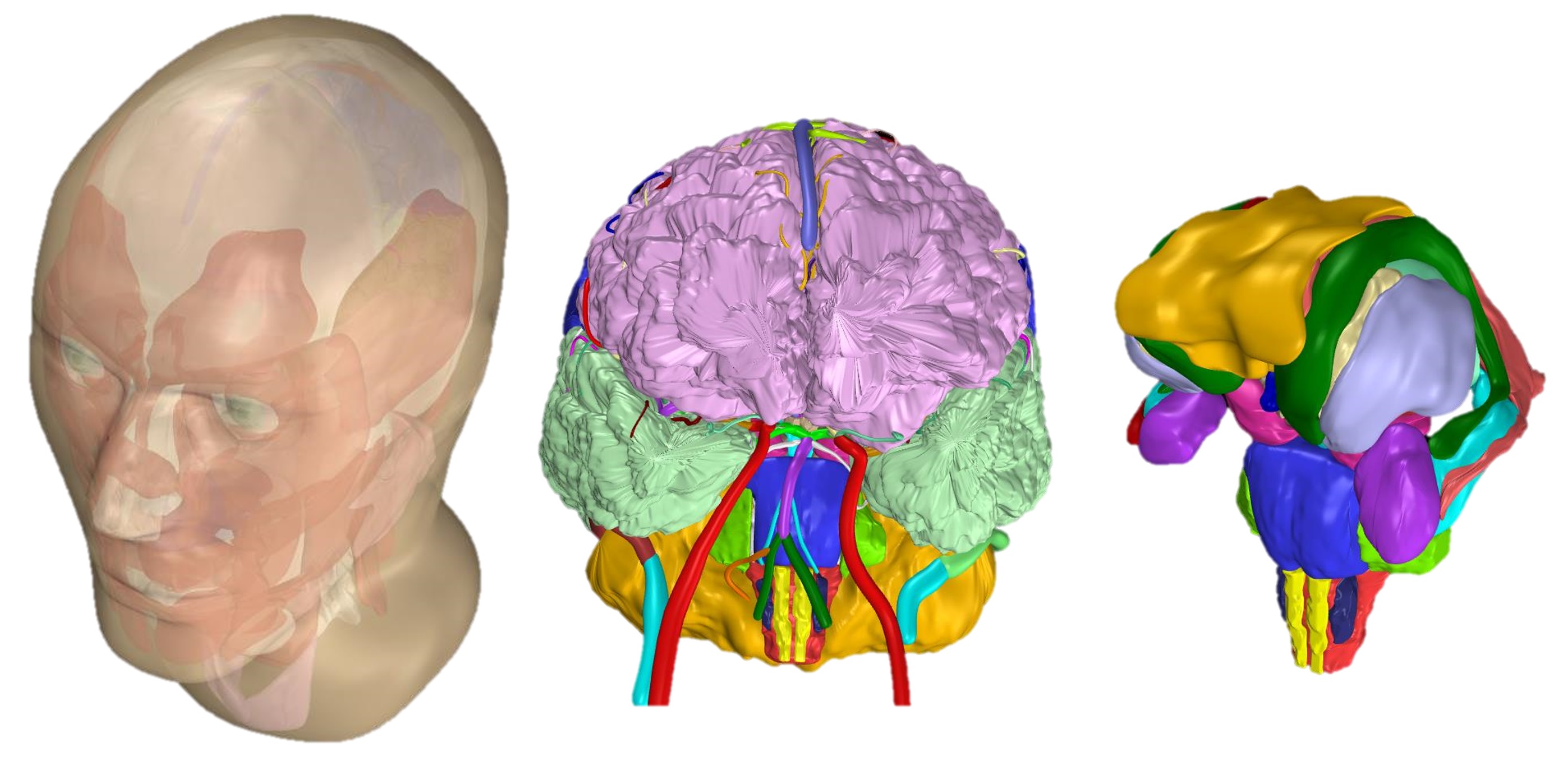
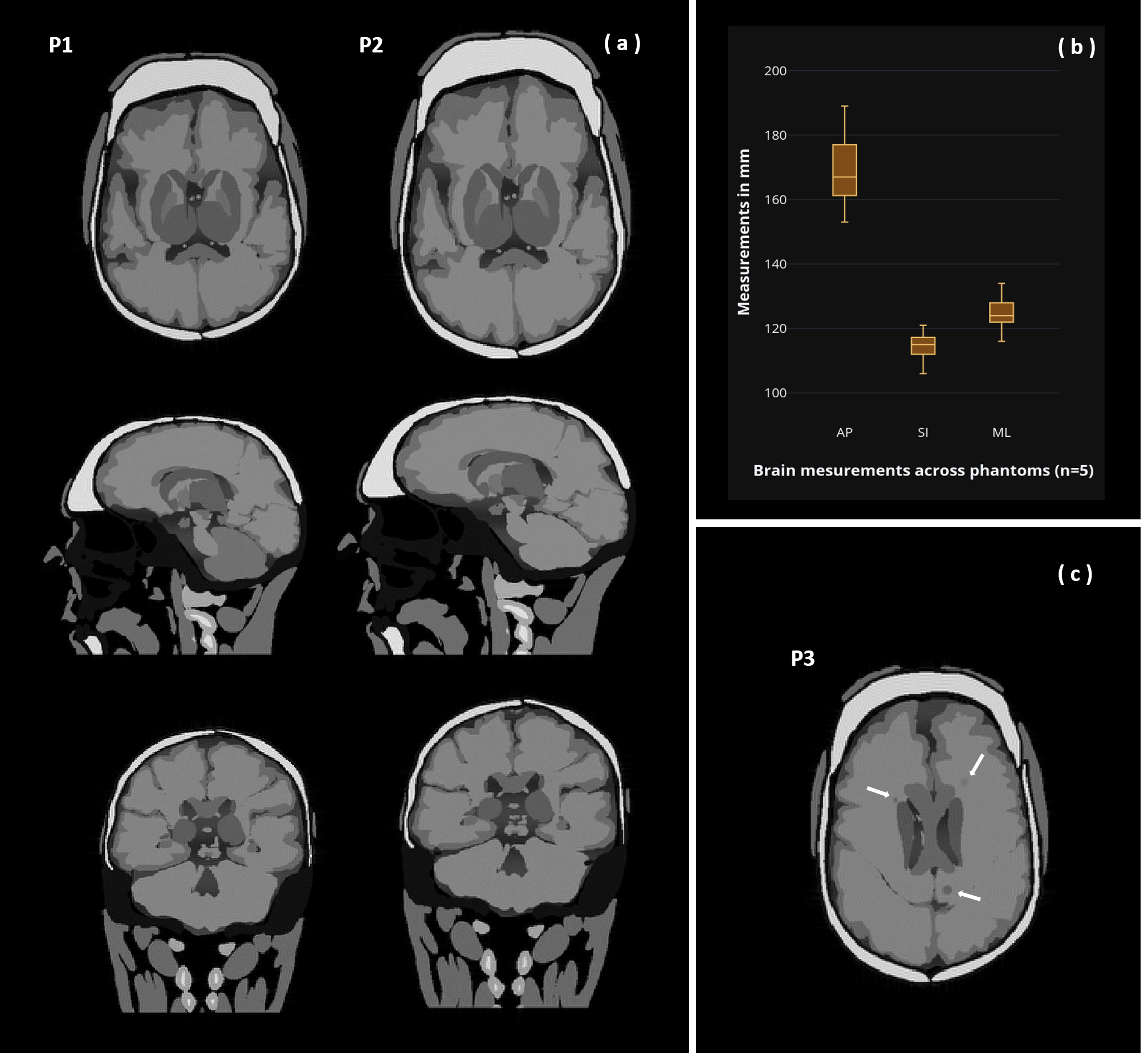
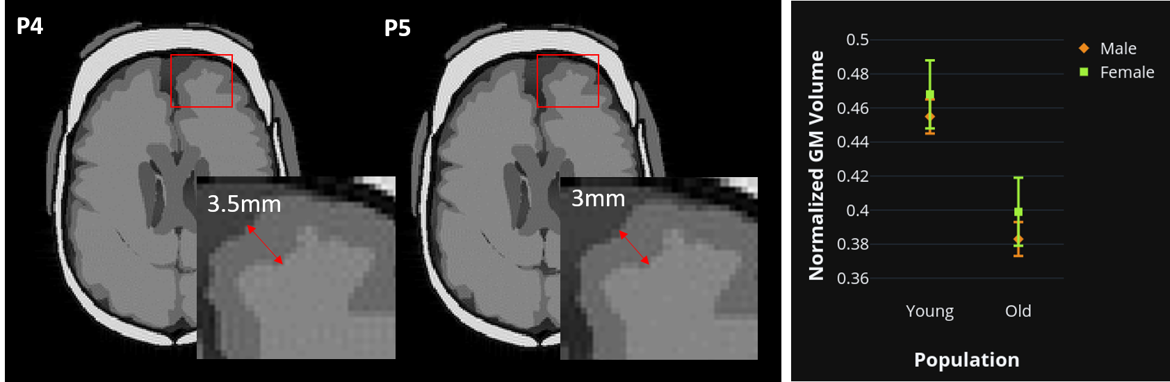
The pipeline designed for simulating realistic brain MRI is shown in Figure 1. The whole body 4D XCAT phantom¹ for multimodality imaging research is used as starting point. The phantom includes highly detailed comprehensive male and female anatomies modeled as NURBS surfaces. The complete head model is shown in Figure 2.
One type of anatomical variation is generated by scaling brain surfaces along anterior posterior, superior inferior and medial lateral directions. Five sets of head phantoms are generated for different brain sizes. Three of the selected scalings relate to the real measurements of subject’s brains from a 3D brain printing study⁵. The other two come from the default XCAT male and female anatomies, which are modelled according to the 50% percentile of US population. Brain measurements utilized across phantoms are presented in Figure 3b. To mimic aging brains, brain cortical Gray Matter (GM) volumes are adapted. Ten sets of head phantoms (five male and five female) with different corresponding GM volumes are generated by extruding and scaling each GM surfaces. Volumetric changes for normalized GM are taken from a study of tissue volumetric changes in young and aging population across gender⁶. Normalized GM measurements utilized across phantoms are presented in Figure 4. Furthermore, a head phantom with three spherical lesions of 3-5mm diameter, present in periventricular white matter is generated.
All generated 16 phantoms are voxelized at an isotropic resolution of 0.5mm³ from the surfaces. For a proof of principle, one slice per phantom in axial, sagittal and coronal view is selected for simulation. Diverse tissue properties from literature^7,8 are assigned to the voxelized phantoms. 2D gradient echo T1w MRI images are simulated using open-source numerical Bloch-solver simulation software, JEMRIS². Sequence parameters used are TE 10ms, TR 400ms and FA 90^o, Sinc RF pulse of 2kHz bandwidth, max gradient strength of 22mT/m, max gradient slew rate of 100T/m/s and a uniform transmit and receive coil is used for simulation sequence design. Cartesian k-space data is simulated at 1mm² resolution from a high resolution phantom model. To include realistic reconstruction, the raw k-space data is fed into the reconstruction pipeline that is used on Philips clinical MRI scanners. Simulated images are qualitatively evaluated for the generated contrast of brain details present, and the reconstruction image quality. To validate GM volumetric changes, cortical thickness is measured across simulated images.

Results

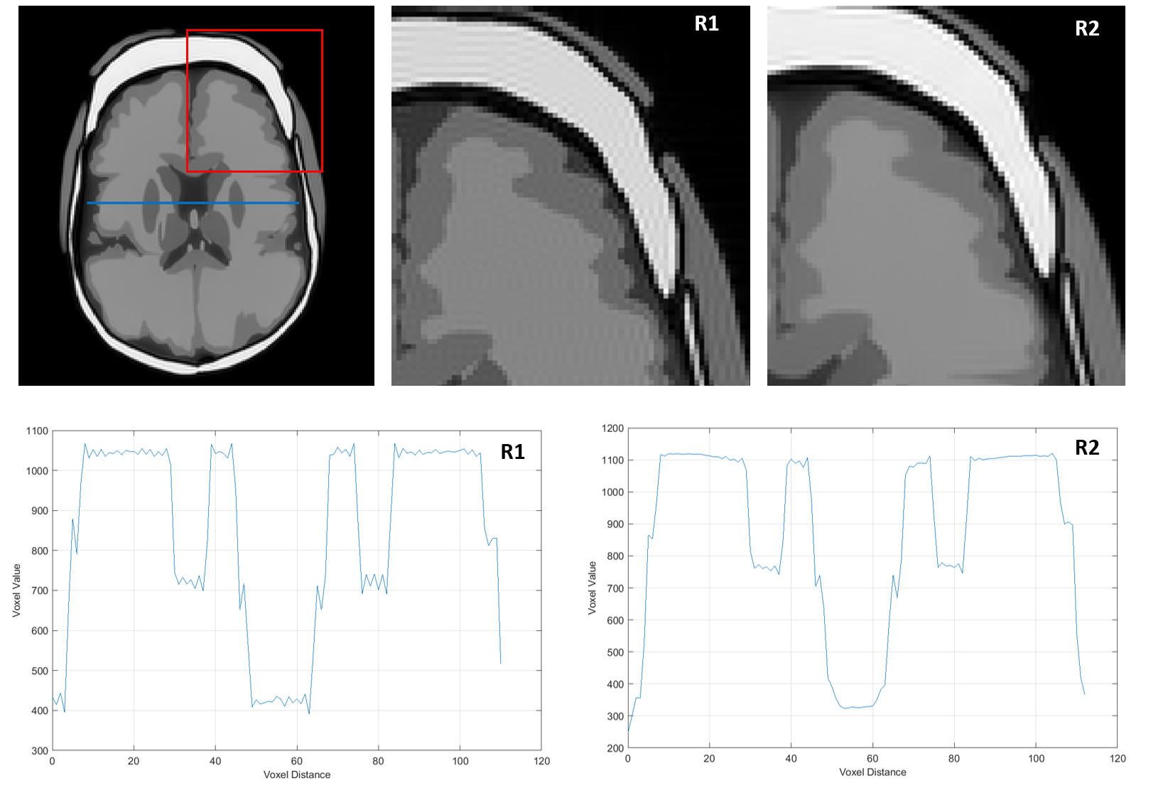
Simulated MRI samples for two (P1-2) full head phantoms with different brain sizes are presented in Figure 3a. In addition to the complete head structures and brain soft tissues, deep gray structures like putamen, thalamus, globus pallidus and caudate nucleus are visible in the slice due to significant contrast generated. In Figure 3c, simulated MRI sample with Multiple Sclerosis lesion (P3) is presented with all lesions visible. Another two (P4-5) simulated MRI samples for different GM volumes are presented in Figure 4. A cortical thickness decrease of 0.5mm in superior frontal gyrus is measured. Per slice simulation took ~20 min on 16 core processor. Reconstruction comparisons of simple FFT (R1) and Philips reconstruction pipeline (R2) for simulated k-space data are presented in Figure 5. Significant reconstruction improvement in R2 is visible as smooth boundaries and reduced Gibbs artifacts.

Discussion and Conclusion

Using this pipeline, all anatomical variations are realistically represented in the simulated images. Detailed brain phantom and true relaxation times for each deep gray structure, has provided a significant contrast for deep gray structures visualization. Using clinically used realistic reconstruction pipeline, has generated simulated images with reduced artifacts, and fine contrasted edges with limited partial volume effects. They contain no variations yet within tissues due to lacking texture information. In addition, no noise and field inhomogeneities were yet been incorporated into our simulations.
In the future, tissue texture information, partial volume and realistic noise need to be incorporated into our pipeline to make simulated image appearance even more realistic. The population of phantom instances has to be enlarged to represent further variability in terms of reflecting normal brain anatomical variations and brain pathologies. A more detailed aging brain with other structural changes corresponding to cortical GM volumetric changes has to be simulated.

Acknowledgements

This work has been supported by openGTN (opengtn.eu) project grant in the EU Marie Curie ITN-EID program (project 764465).