Introduction

Cerebral microbleeds (CMBs) are known risk factors of stroke and hemorrhage that can be a marker of cognitive impairment. Although CMBs are easily visualized with susceptibility weighted imaging (SWI), they are burdensome to localize and quantify manually. Image processing algorithms based on the radial symmetry transform have previously been used to identify candidate CMBs^1,2, and convolutional neural networks (CNNs) have been effective at distinguishing real CMBs from their false positive mimics with high sensitivity and specificity^3,4. The goal of this study was to train a deep neural network to carry out this entire processing pipeline and to predict CMB voxel masks using a dataset of radiation therapy-induced CMBs from patients with gliomas.

Methods

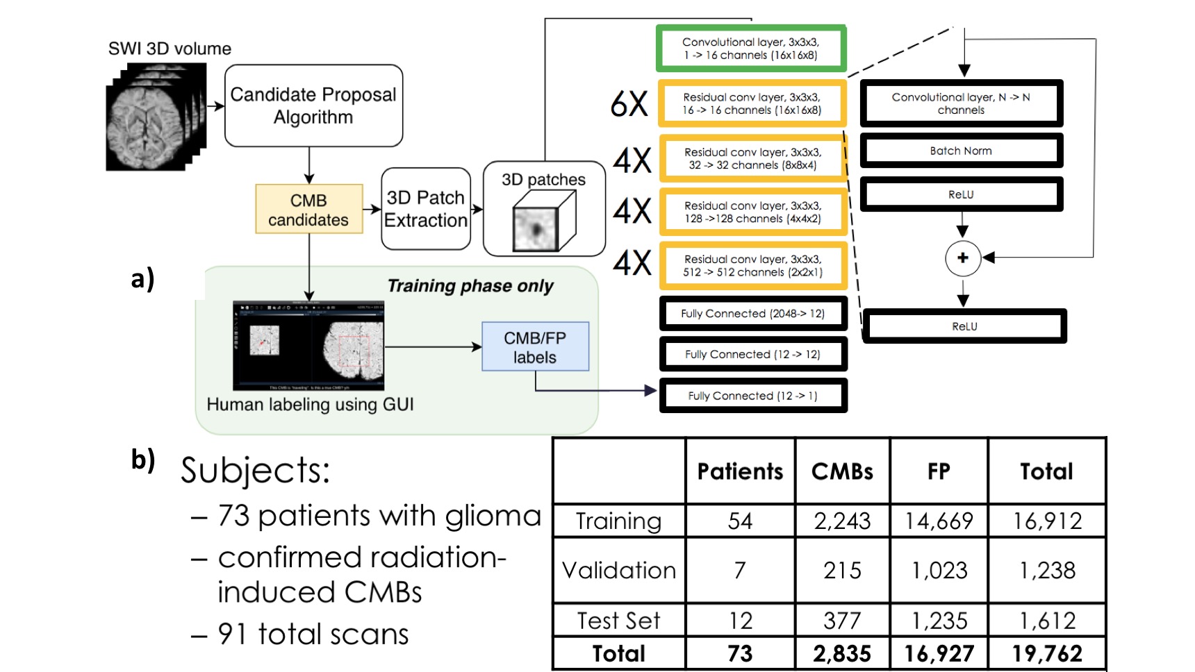
Dataset: 7T SWI scans of brain tumor patients with radiation induced CMBs were acquired on a GE 7T scanner equipped with a 32-channel receive coil using either a standard SWI sequence (resolution = 0.5x0.5x2mm, FOV. = 24x24cm, TE = 16ms, TR = 50ms, 49 subjects) or a 4-echo 3D TOF-SWI sequence⁵ (resolution=0.5x0.5x1mm, TE = 2.7, 10.4, 13.2, 20.9 ms, TR = 40ms, 31 subjects). Figure 1b shows the breakdown of the number of patients, exams, and CMBs in each of the training, validation, and test datasets.

Pre-processing: To acquire a labeled dataset to pre-train the network, the SWI scans were initially processed with a fast radial symmetry transform algorithm¹ to find candidate CMBs, which were then inspected using a user-friendly GUI2 before segmenting the resulting candidate CMBs and false-positive mimics. The center coordinates of these labeled masks were then used to extract 16 x 16 x 8 3D patches to use as inputs to the ResNet CNN as shown in Figure 1a, with the target output of 1 corresponding to a true CMB patch. For the mask segmentation training, the same CMB and mimic input patches were used, along with their corresponding segmented labeled masks as target outputs.

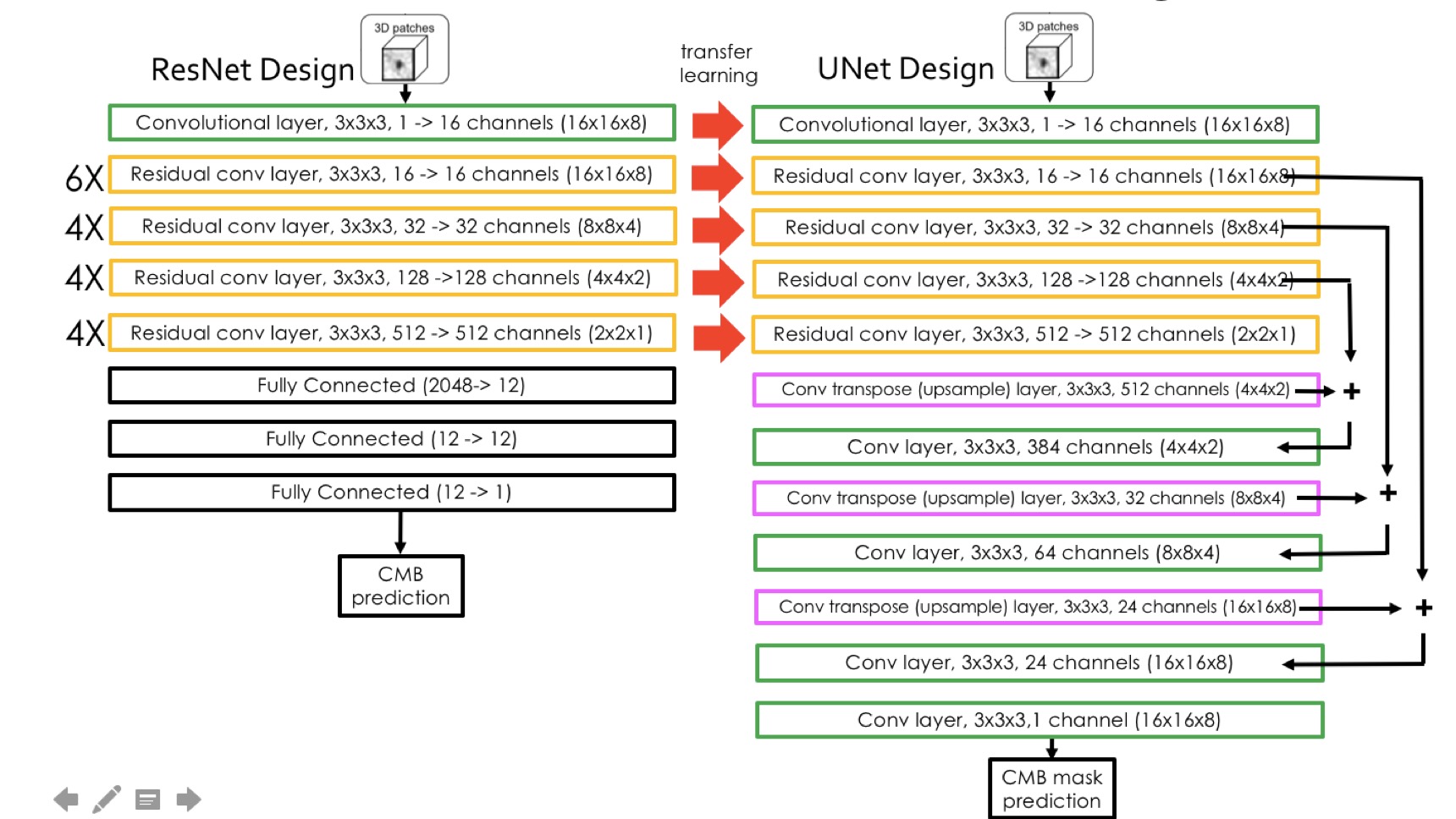
Deep network model strategy: A ResNet architecture with 3D convolutional kernels³ followed by fully connected blocks was first trained to classify voxel patches as containing either a CMB or a mimic feature. The residual blocks from this network were then used as the pre-trained front end for a UNet architecture that was subsequently trained to generate segmented voxel masks for CMB patches as shown in Figure 2. The network was trained using a Nvidia Titan Xp GPU with 12GB memory and the Adam optimizer that began with a learning rate of 0.001 and experienced a cosine decay over each epoch for ~100,000 iterations. A batch size of 32 was utilized and a weighted binary cross entropy was employed as the loss function, where the weight was equal to the number of voxels that were part of a CMB divided by the total number of voxels in the training set. In order to avoid overfitting, data augmentation including random rotations and flips was carried out.

Results and Discussion

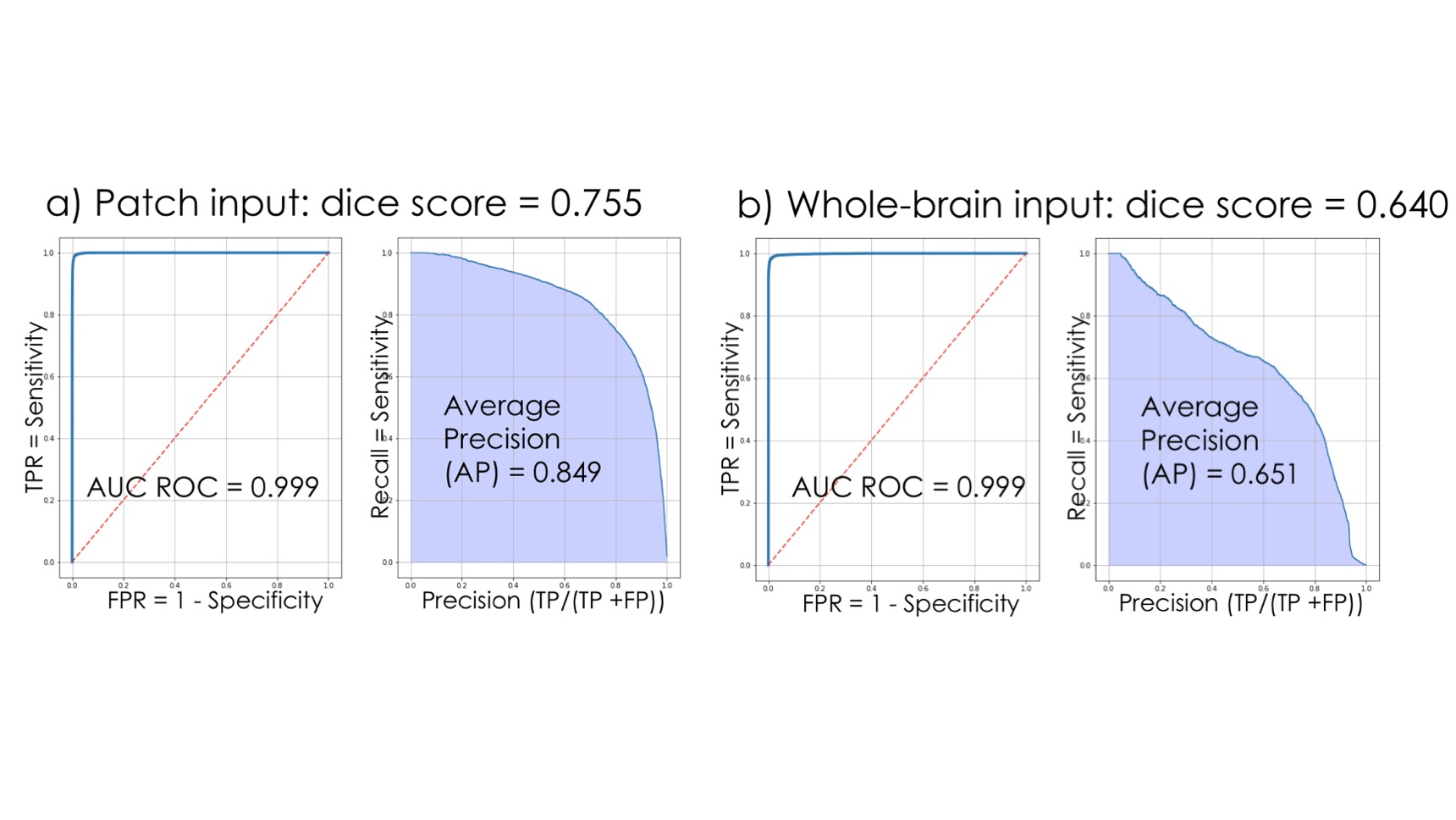
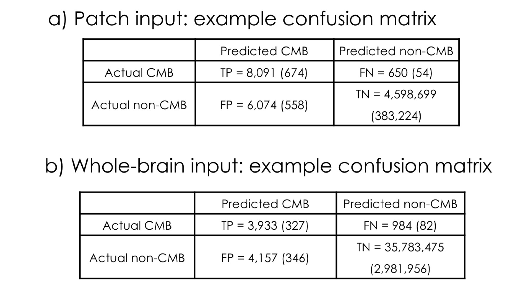
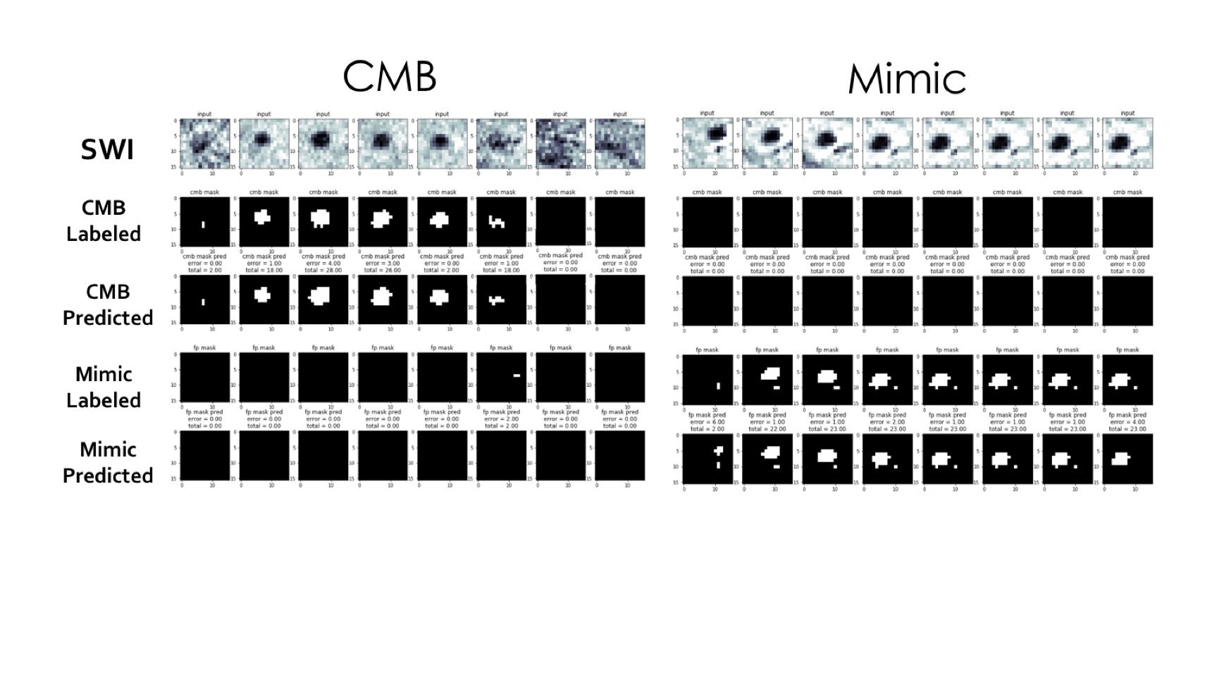
The classification network used in pre-training achieved an ROC area under curve (AUC) of 97.7% and an average precision of 93.5%. Figures 3 shows the Receiver Operating Characteristic (ROC) and Precision-Recall curves for the results of the mask segmentations. The mask prediction network achieved a dice score of 0.755 on patched-based predictions, but only 0.644 when given the whole brain at once in testing. The corresponding confusion matrices are shown in Figure 4. A comparison of the network predictions for two representative CMB and mimic masks for two extreme cases with very large CMB/mimic features is illustrated in Figure 5.

After the UNet has been trained to predict CMB voxel masks, it can still be used to classify patches by checking to see if any voxel in a patch has a predicted likelihood of being a CMB above a threshold. Using this method, the ROC AUC is 95.7% and the average precision is 84.8%, with only 12.6 false-positive CMB mimics per patient. Although the classification performance was reduced compared to the original classification architecture, the mask prediction task is different because it must learn 3D position information about CMBs and it requires a much larger network to reach the same performance standard as the classifier. Including a second input channel corresponding to the phase image⁴ during training did not improve classification or mask prediction performance.

The whole brain prediction utilizes test-time augmentation where the input data is flipped and rotated in a number of ways such that 32 different predictions for the same brain are averaged together. This augmentation provided a benefit in mask prediction precision but extends the total computation time on a Titan XP GPU to 80 seconds as opposed to 30 seconds without augmentation.

Conclusion

In spite of the apparently obvious appearance of CMB features on SWI images, segmenting accurate CMB masks that exclude mimic features is difficult. We trained a UNet architecture to predict the positions of CMB voxels on a large dataset of SWI patches, and demonstrated high sensitivity and specificity on test sets of patch-based inputs. The high performance and short computation time of the network for automating CMB quantification point toward a possible clinical application.

Acknowledgements

Funding Information: this work was supported by the National Institute for Child Health and Human Development of the National Institutes of Health grant R01HD079568 and GE Healthcare.