1867
Using an Artificial Neural Network for Fast Mapping of the Oxygen Extraction Fraction with Combined QSM and qBOLD1Computer Assisted Clinical Medicine, Heidelberg University, Mannheim, Germany, 2Department of Biomedical Engineering, Cornell University, Ithaca, NY, United States, 3Department of Radiology, Weill Cornell Medical College, New York, NY, United States, 4Department of Radiology, Tongji Hospital, Wuhan, China
Synopsis
MRI-based mapping of the oxygen extraction fraction (OEF) is a valuable addition to diagnosis and treatment planning of various diseases; yet, it often lacks robustness and suffers from elaborate, time-consuming reconstructions. We trained an artificial neural network (ANN) on simulated QSM values and qBOLD data, tested it in 7 healthy volunteers and compared it to a standard quasi-Newton approach. The ANN reduced the intersubject variability of OEF by regularizing the reconstruction. Moreover, it lowered the reconstruction time from approximately one hour to one second and removed the necessity of accurate parameter initialization through an additional acquisition.
Introduction
The oxygen extraction fraction (OEF) is a valuable biomarker for tissue vitality and viability in various pathologies.1,2 Yet, current MRI-based OEF mapping techniques are based on traditional time-consuming iterative reconstructions and have difficulties to robustly separate the underlying model parameters.3 Moreover, they commonly require accurate parameter initialization, which often has to be obtained from additional acquisitions.3 Today, artificial neural networks (ANNs) are widely utilized in general image reconstruction problems4,5 and also allow for highly efficient and robust curve-fitting.6,7 Hence, the aim of this study was to apply an ANN for fast and robust quantification of the oxygen extraction fraction (OEF) from a combined quantitative susceptibility mapping (QSM) and quantitative BOLD (qBOLD) analysis of gradient echo data in the brain and to compare the ANN to a traditional quasi-Newton (QN) method3 for numerical optimization.Methods
Random combinations of venous oxygen saturation $$$Y=Y_\text{a}(1-\text{OEF})$$$, deoxygenated blood volume $$$\nu$$$, $$$R_2$$$ and non-blood susceptibility $$$\chi_\text{nb}$$$ with each parameter following a Gaussian distribution that represented physiological gray and white matter values were used to simulate qBOLD signals for a multi gradient echo sequence with clinical parameter settings.3 The initial magnitude signal $$$S_0$$$ was normalized so that $$$S(\text{TE}_1)=1$$$. The same combinations of $$$Y$$$, $$$\nu$$$ and $$$\chi_\text{nb}$$$ were utilized to simulate QSM values.3 An ANN was trained on the simulated data with added Gaussian noise using the Neural Network toolbox of Matlab 2017a (MathWorks, Natick, MA, USA). The ANN was applied to multi-gradient echo brain data of 7 healthy subjects, and the reconstructed parameters and maps were compared to QN results using Student’s t-test and Bland-Altman analysis. The QN approach used an initialization $$$\nu_\text{start}$$$ for the deoxygenated blood volume that was estimated from an arterial spin labelling sequence by an empirical relationship.8,3Results
The distributions of training parameters and the training performance of the network are illustrated in Figure 1. Figure 2 depicts a representative slice of the $$$\text{OEF}=1-Y/Y_\text{a}$$$ from the ANN and QN reconstruction. The same slice of the remaining model parameters is illustrated in Figure 3 including $$$\nu_\text{start}$$$. Intersubject means and standard deviations of gray matter were $$$\text{OEF}=43.5\pm0.8\,\%$$$, $$$R_2=13.5\pm0.3\,\text{Hz}$$$, $$$\nu=3.4\pm0.1\,\%$$$, $$$\chi_\text{nb}=-25\pm5\,\text{ppb}$$$ for ANN and $$$\text{OEF}=43.8\pm5.2\,\%$$$, $$$R_2=12.2\pm0.8\,\text{Hz}$$$, $$$\nu=4.2\pm0.6\,\%$$$, $$$\chi_\text{nb}=-39\pm7\,\text{ppb}$$$ for QN with a significant difference (p<0.05) for $$$R_2$$$, $$$\nu$$$ and $$$\chi_\text{nb}$$$. Of white matter, it was $$$\text{OEF}=47.5\pm1.1\,\%$$$, $$$R_2=17.1\pm0.4\,\text{Hz}$$$, $$$\nu=2.5\pm0.2\,\%$$$, $$$\chi_\text{nb}=-38\pm5\,\text{ppb}$$$ for ANN and $$$\text{OEF}=42.3\pm5.6\,\%$$$, $$$R_2=16.7\pm0.7\,\text{Hz}$$$, $$$\nu=2.9\pm0.3\,\%$$$, $$$\chi_\text{nb}=-45\pm9\,\text{ppb}$$$ for QN with a significant difference (p<0.05) for $$$\text{OEF}$$$ and $$$\nu$$$. Boxplots showing the intersubject variability are given in Figure 4. ANN revealed more gray-white matter contrast but less intersubject variation in $$$\text{OEF}$$$ than QN. Bland-Altman plots for all reconstructed parameters from the two methods are depicted in Figure 5. In contrast to QN, the ANN reconstruction did not need an additional sequence for parameter initialization and took approximately one second rather than roughly one hour.Discussion
The ANN implemented here regularizes the reconstruction, which is illustrated by the negative linear trend visible in the Bland-Altman plots and the reduced intersubject variation especially for the OEF. Yet, it removes the necessity of parameter initialization from an additional sequence and strongly accelerates the reconstruction. This might facilitate a clinical implementation of QSM+qBOLD for OEF reconstructions. The standard deviation for the training parameters used here was chosen to reflect the variation expected in healthy volunteers. However, it also determines the tradeoff between increased robustness and sensitivity to subtle parameter changes of the QSM+qBOLD reconstruction. Whether the advantages of higher robustness and speed observed with the ANN come at the cost of lower sensitivity for subtle OEF changes in diseases such as stroke and brain tumors, remains to be investigated in future clinical studies.Conclusion
ANNs allow faster and with regard to initialization more robust reconstruction of OEF maps with lower intersubject variation than QN approaches.Acknowledgements
No acknowledgement found.References
1. Vaupel P, Mayer A. Hypoxia in cancer: significance and impact on clinical outcome. Cancer Metastasis Rev 2007;26(2):225-239.
2. Ibaraki M, Shimosegawa E, Miura S, Takahashi K, Ito H, Kanno I, Hatazawa J. PET measurements of CBF, OEF, and CMRO2 without arterial sampling in hyperacute ischemic stroke: method and error analysis. Ann Nucl Med 2004;18(1):35-44.
3. Hubertus, S, Thomas, S, Cho, J, Zhang, S, Wang, Y, Schad, LR. Comparison of gradient echo and gradient echo sampling of spin echo sequence for the quantification of the oxygen extraction fraction from a combined quantitative susceptibility mapping and quantitative BOLD (QSM+qBOLD) approach. Magn Reson Med 2019;82:1491-1503.
4. Yoon J, Gong E, Chatnuntawech I, et al. Quantitative susceptibility mapping using deep neural network: QSMnet. Neuroimage 2018;179:199-206.
5. Hammernik K, Klatzer T, Kobler E, Recht MP, Sodickson DK, Pock T, Knoll F. Learning a variational network for reconstruction of accelerated MRI data. Magn Reson Med 2018;79(6):3055-3071.
6. Bertleff M, Domsch S, Weingärtner S, Zapp J, O'Brien K, Barth M, Schad LR. Diffusion parameter mapping with the combined intravoxel incoherent motion and kurtosis model using artificial neural networks at 3 T. NMR Biomed 2017;30(12):e3833.
7. Domsch S, Murle B, Weingartner S, Zapp J, Wenz F, Schad LR. Oxygen extraction fraction mapping at 3 Tesla using an artificial neural network: A feasibility study. Magn Reson Med 2018;79:890-899.
8. Leenders KL, Perani D, Lammertsma AA, et al. Cerebral blood flow, blood volume and oxygen utilization. Normal values and effect of age. Brain 1990;113(1):27-47.
Figures
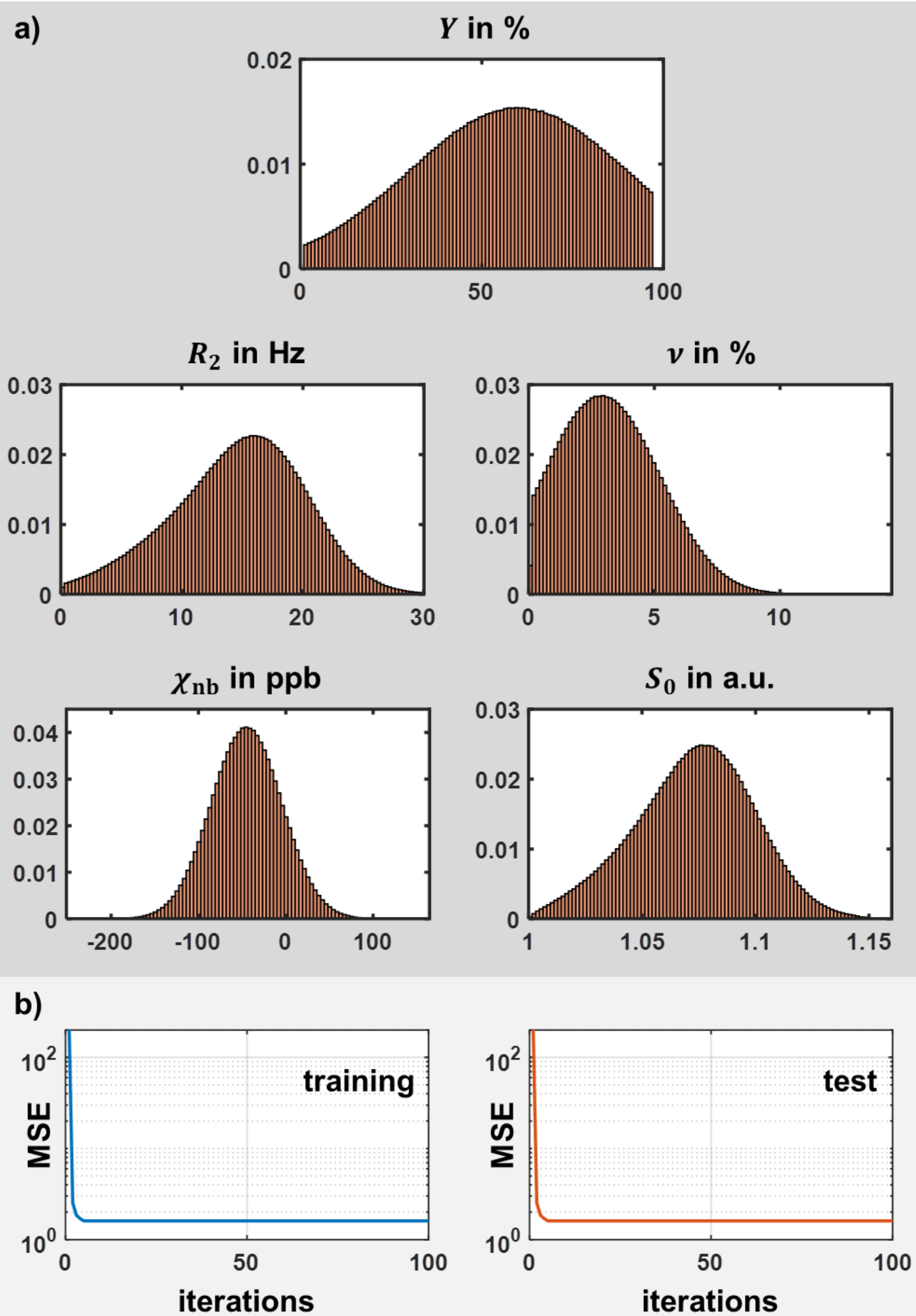
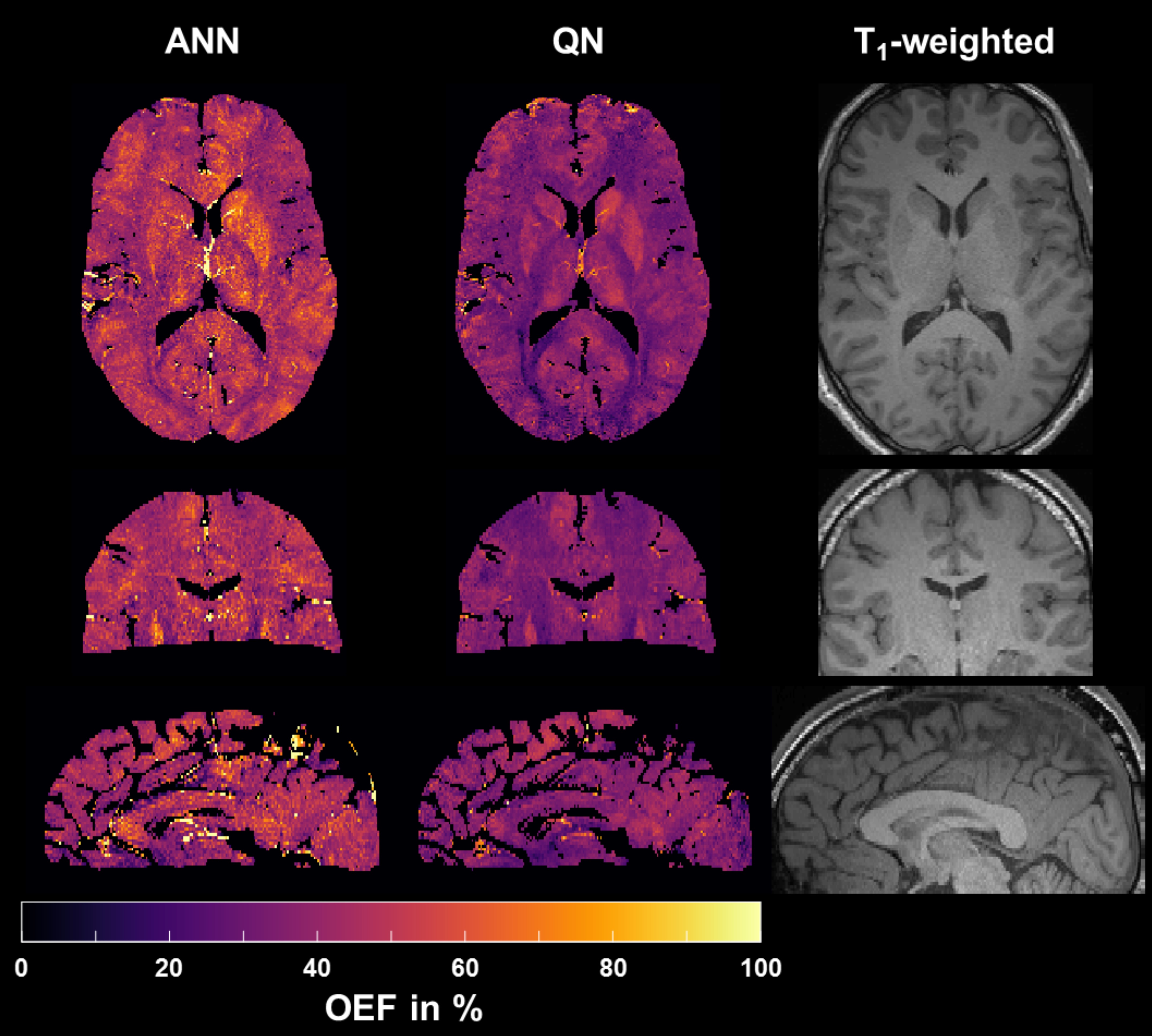
Figure 2: Representative axial, coronal and sagittal slice of the oxygen extraction fraction $$$\text{OEF}$$$ reconstructed with the artificial neural network (ANN) and quasi-Newton (QN) approach. The corresponding T1-weighted morphological reference image is given on the right.
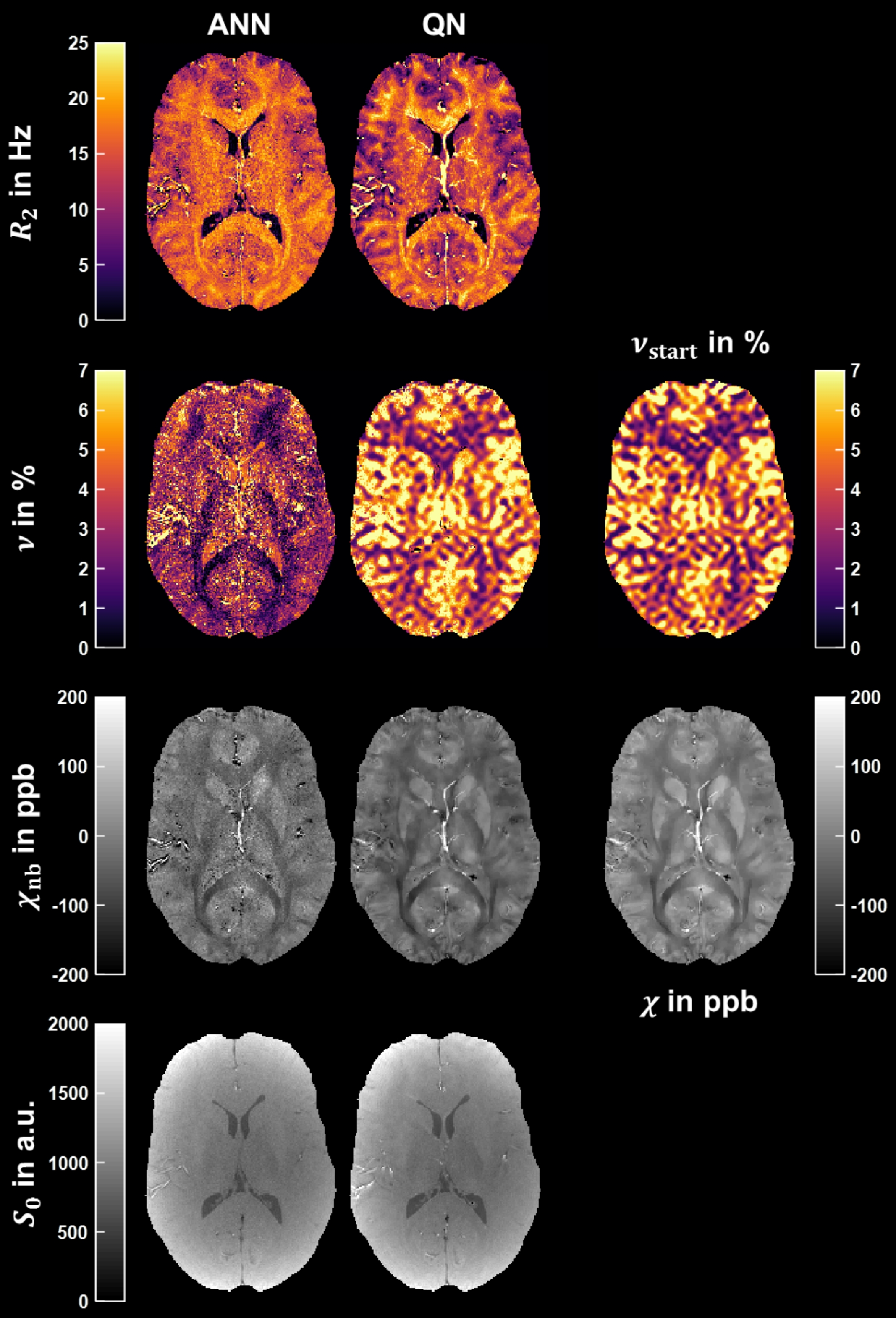
Figure 3: Representative axial slice of the transverse relaxation rate $$$R_2$$$, deoxygenated blood volume $$$\nu$$$, non-blood magnetic susceptibility $$$\chi_\text{nb}$$$ and magnitude after excitation $$$S_0$$$ reconstructed using the artificial neural network (ANN) and quasi-Newton (QN) method. The corresponding slice of $$$\nu_\text{start}$$$ used for initialization and the magnetic susceptibility $$$\chi$$$ from QSM used for the final QN fit are pictured on the right. The axial slice is the same as in Figure 2.
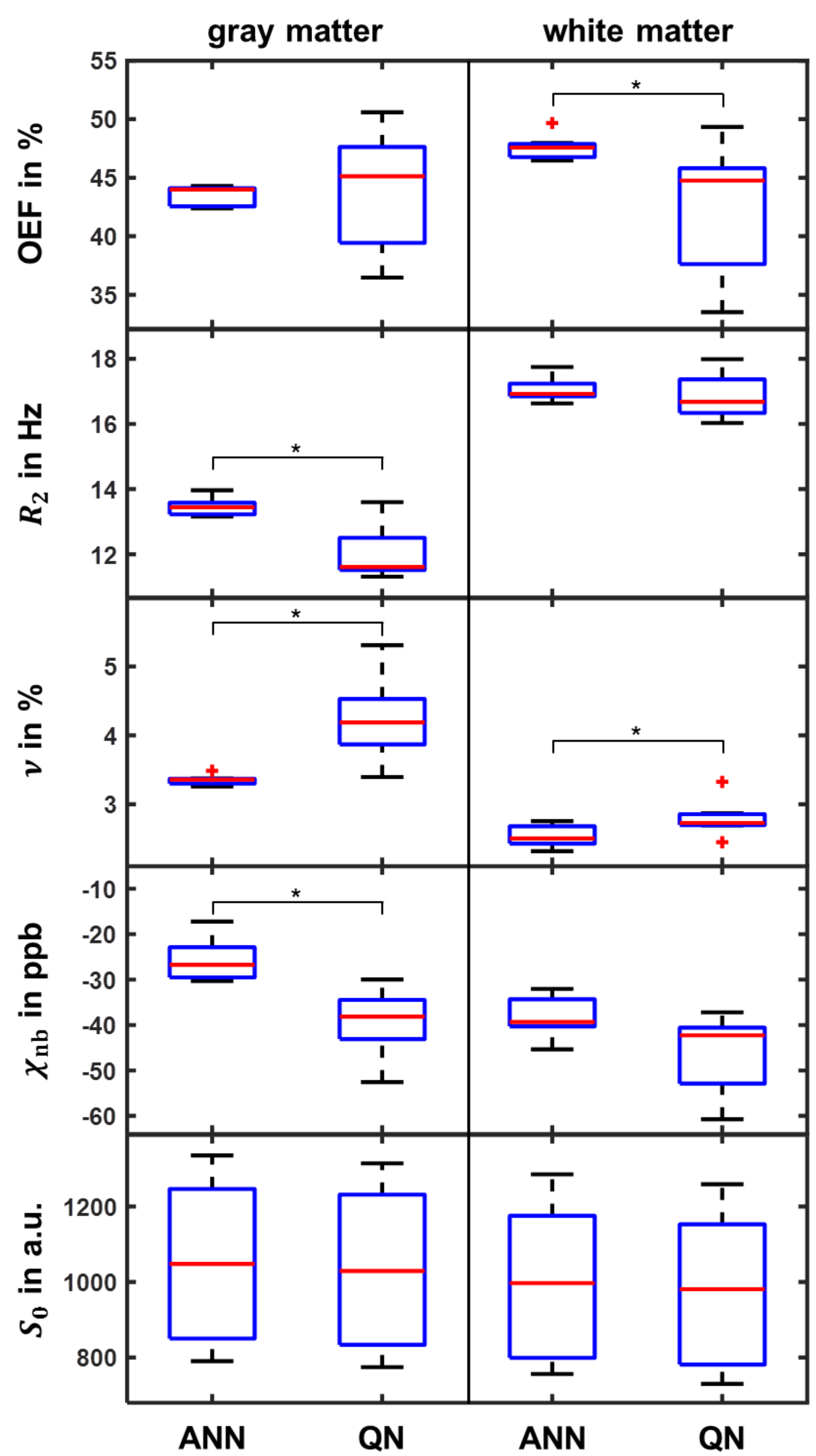
Figure 4: Boxplot illustrating intersubject variability within gray (left) and white matter (right) for $$$\text{OEF}$$$, $$$R_2$$$, $$$\nu$$$, $$$\chi_\text{nb}$$$ and $$$S_0$$$ reconstructed using the artificial neural network (ANN) and quasi-Newton (QN) method. Depicted are median (red), first and third quartile (blue) and whiskers at 1.5 times the interquartile distance (black). Significant differences (p<0.05) between the approaches are marked with an asterisk.
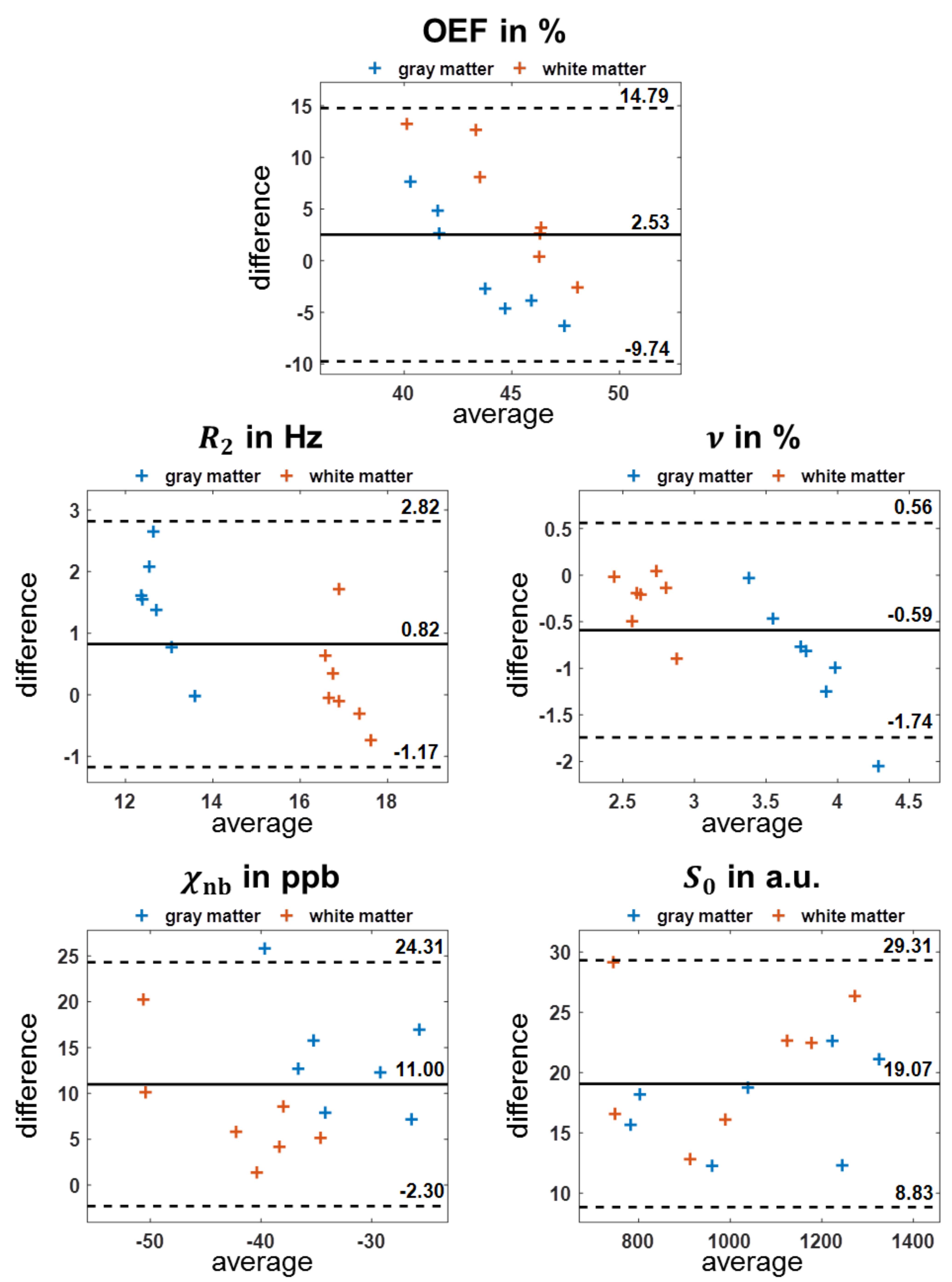
Figure 5: Bland-Altman plots comparing artificial neural network (ANN) and quasi-Newton (QN) approach for the oxygen extraction fraction $$$\text{OEF}$$$, transverse relaxation rate $$$R_2$$$, deoxygenated blood volume $$$\nu$$$, non-blood magnetic susceptibility $$$\chi_\text{nb}$$$ and magnitude after excitation $$$S_0$$$ within gray (blue) and white matter (orange) in all 7 subjects. Plotted are difference=xANN-xQN over average=(xANN+xQN)/2 as well as the mean (black line) and mean±1.96·standard deviation (black dashed lines).