Introduction

Quantitative MR-imaging methods, such as MR Fingerprinting(MRF)¹ and MRF-EPI², are used to measure tissue properties (e.g. FISP-MRF³:T₁,T₂; MRF-EPI²: T₁,T₂^*) and can therefore be used to derive standard and novel MRI-biomarkers. Common quantitative MR methods assume a single set of relaxation properties per voxel. However, this is not valid in the presence of partial volume effects as well as in tissues consisting of multiple components. Sensitivity to such multi-component effects in and around lesions can also provide more insight into disease processes.

In the brain of healthy subjects a small number of tissues is expected and multi-component MRF(MC-MRF) using (global) joint-sparsity⁴ with the SPIJN algorithm, can be used to obtain a partial volume segmentation of the different components. Due to the highly correlated MRF-dictionary SPIJN is able to identify around ten tissues. However, tissue properties of small cerebral lesions can vary per lesion and lesions occur in small regions, making the global joint sparsity less applicable. Voxel-wise methods^5,6 without joint sparsity constraints, on the other hand, show lower noise resilience.

In this work, we develop a MC-MRF algorithm based on a joint sparsity constraint that is applied locally to be particularly sensitive to small pathologies. As a proof of principle, this method is used for automatic lesion detection in MRF-EPI data from a patient with MS.

Methods

The Sparsity Promoting Iterative Joint NNLS (SPIJN) algorithm⁴ was extended in order to account for small structures. The resulting local-SPIJN algorithm is based on the premise that a local region only consists of a small number of components.
Hence, we solved the following minimization problem:$$\min_{C\in\mathbb{R}_{\geq 0}^{N\times\,J}}\left\lVert X-DC\right\rVert_2^F\\\text{s.t.}\left\lVert\,C_{R(v_j)}\right\rVert_{r}\,\text{is small}\,\forall\,j\in\{0,...,J\}$$where X is a matrix containing the J measured signals, D the MRF-dictionary and C a matrix containing the N component weights for every voxel. $$$C_{R(v_j)}$$$ denotes the submatrix of C consisting of the subset R of voxels in the vicinity of voxel j. $$$\left\lVert\cdot\right\rVert_r$$$ counts the number of non-zero rows of a matrix.
We solved the problem iteratively based on the NNLS-algorithm⁷, with the following iterations:
$$R=\operatorname{diag}\left(\left(\mathbf{w}^{k+1}_j\right)^{1/2}\right),\\\tilde{D}=\begin{bmatrix}DR\\\lambda\mathbf{1}^T\end{bmatrix},\\\mathbf{\tilde{x}}=\begin{bmatrix}\mathbf{x}_{j}\\0\end{bmatrix},\\\tilde{\mathbf{c}}=\min_{c\in\mathbb{R}_{\geq 0}^{N}}\left\lVert\mathbf{\tilde{x}}-\tilde{D}\mathbf{c}\right\rVert_2,\\\mathbf{c}^{k+1}_j= R\tilde{\mathbf{c}}.$$Notably, weights $$$\mathbf{w}^{i,k+1}$$$ were calculated by spatial Gaussian smoothing of the previous solution $$$c^i$$$(row $$$i$$$ of $$$C$$$) for tissue $$$i$$$. The standard deviation $$$\sigma$$$ of the Gaussian essentially governed the locality. $$$\lambda=0.8,\,\sigma=[4,4,4/2]\,$$$px$$$\,=[4,4,4]\,$$$mm(in x,y,z-direction) were used in this study.
MRF-EPI² was used to test the method in numerical experiments and in-vivo. A dictionary with T₁=30ms-4s,T₂^*=5ms-3s(5% increase) and B₁=0.65-1.35(0.05 stepsize) was used.

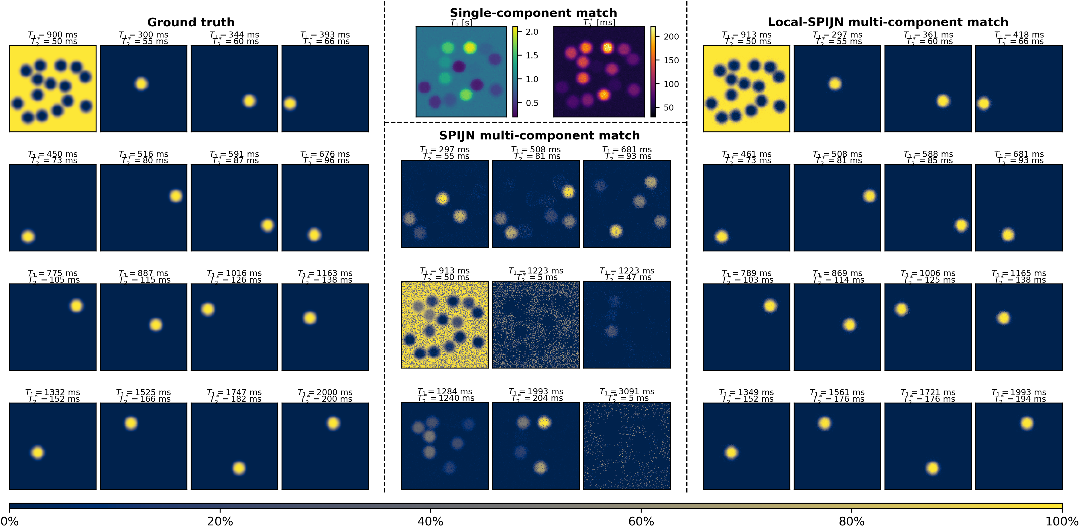
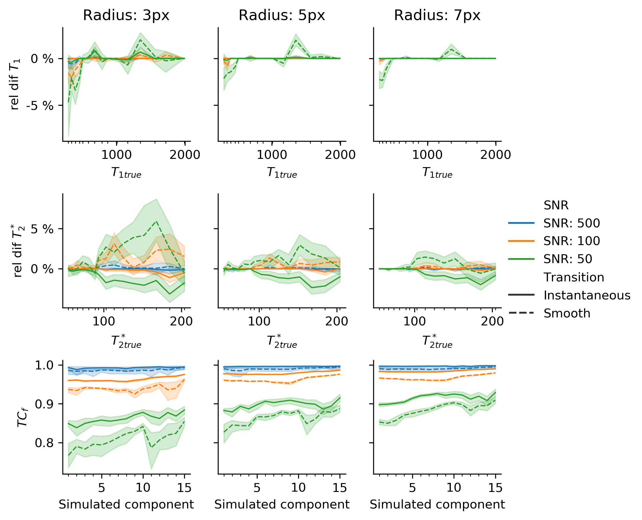
A numerical phantom of size $$$100\times100$$$ pixels consisting of a background tissue with T₁=900ms,T₂^*=50ms (representing white matter) and 15 non-overlapping randomly placed dot-shaped abnormalities with log-distributed T₁,T₂^*(300ms-2s,55ms-200ms resp.) was used to test the local-SPIJN algorithm. Transitions between background and dots were either smooth or instantaneous. Varying SNR(50,100,500) and radii(3,5,7px) were used.
Resulting partial volume segmentations $$$B$$$ from the proposed local-SPIJN algorithm were compared to the ground truth $$$A$$$ through the fuzzy Tanimoto coefficient⁸: $$$TC_F=\frac{\sum_{i\in\textit{pixels}}\textit{MIN}(A_i,B_i)}{\sum_{i\in\textit{pixels}}\textit{MAX}(A_i,B_i)}$$$.

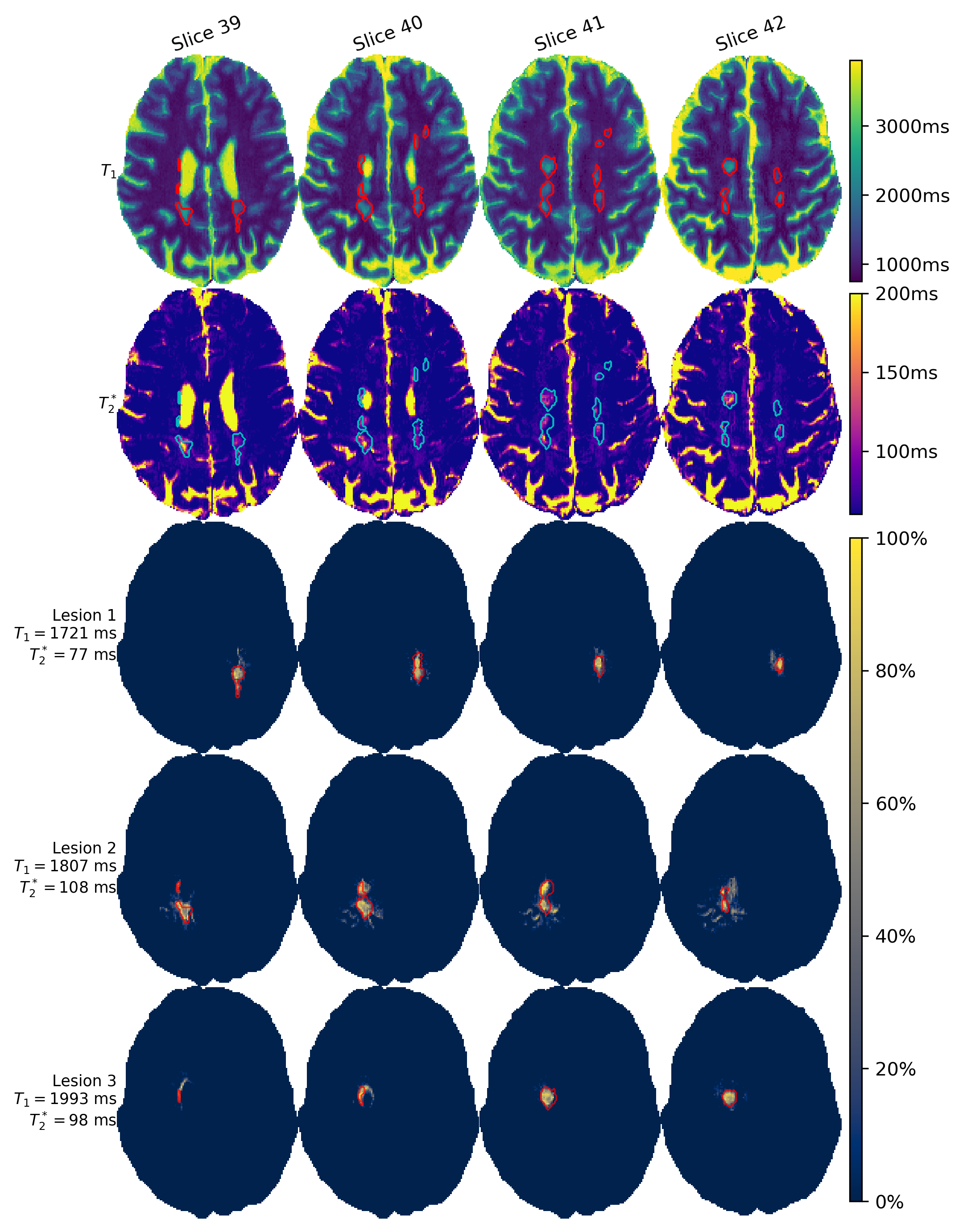
The proposed algorithm was applied to MRF-EPI data acquired from a patient with MS (resolution $$$1\times\,1\times\,2$$$mm³,$$$\,240\times\,240\times\,60$$$ voxels, acquisition time 1:52 minutes). Components with 1.5s<T₁<2.25s, 75ms<T₂^*<1s were considered as potential lesions, based on increased T₂^*9,10. Results are shown for 4 slices in which lesions were manually segmented by an expert radiologist on FLAIR images.

Results and discussion

Single-component MRF, SPIJN-MC-MRF and the proposed method were compared on one of the numerical phantoms(Fig.1). Single component matching incorrectly resulted in a smooth transition in relaxation times at the borders of the structures. SPIJN-MC-MRF resulted in 2 noisy component and 7 components erroneously not confined to single lesions. The proposed method is able to detect the different lesions in isolation.

Simulation results of the proposed algorithm showed good agreement with the reference for SNR$$$\geq$$$100 (error $$$T_1<1\%,\,T_2^*<2\%,\,{TC}_f>0.92$$$)(Fig.2). SNR=50 gave segmentations of reasonable quality ($$${TC}_f>0.75$$$)⁸.

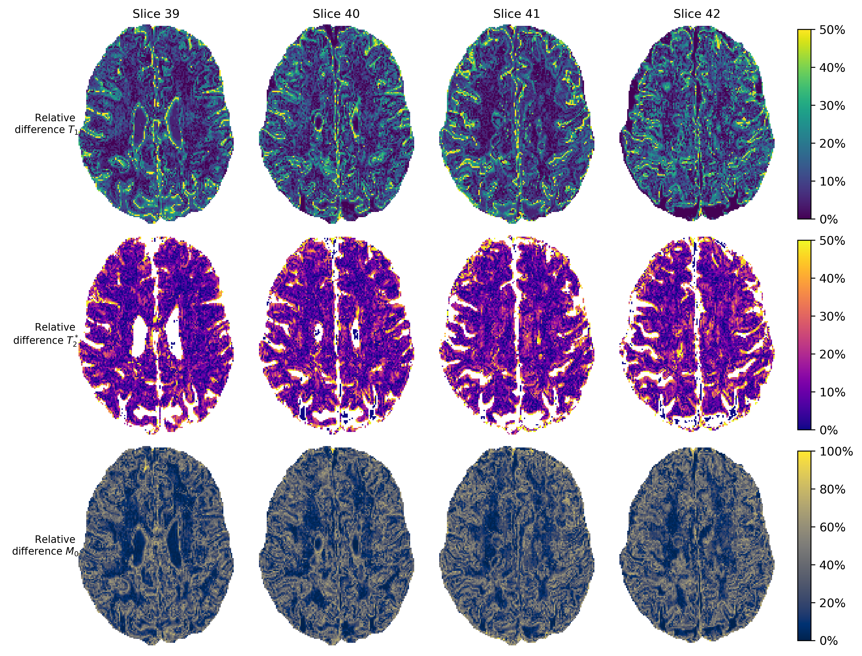
Fig.3 shows relative differences between the M₀,T₁ and T₂^* maps from a single component approach compared to the primary (largest) MC-MRF component. Note the small differences in the white matter (no partial volume) and increased differences around tissue boundaries, where partial volume occurs.
Fig.4 shows T₁-T₂^*-maps obtained from matching and signal fractions of the three components identified as lesions. Note how the detected lesions correspond to lesions as annotated in the quantitative maps. The smaller lesions had relaxation times in the range of gray matter (data not shown). To detect these lesions as well, inclusion of spatial information or other contrasts would be required.

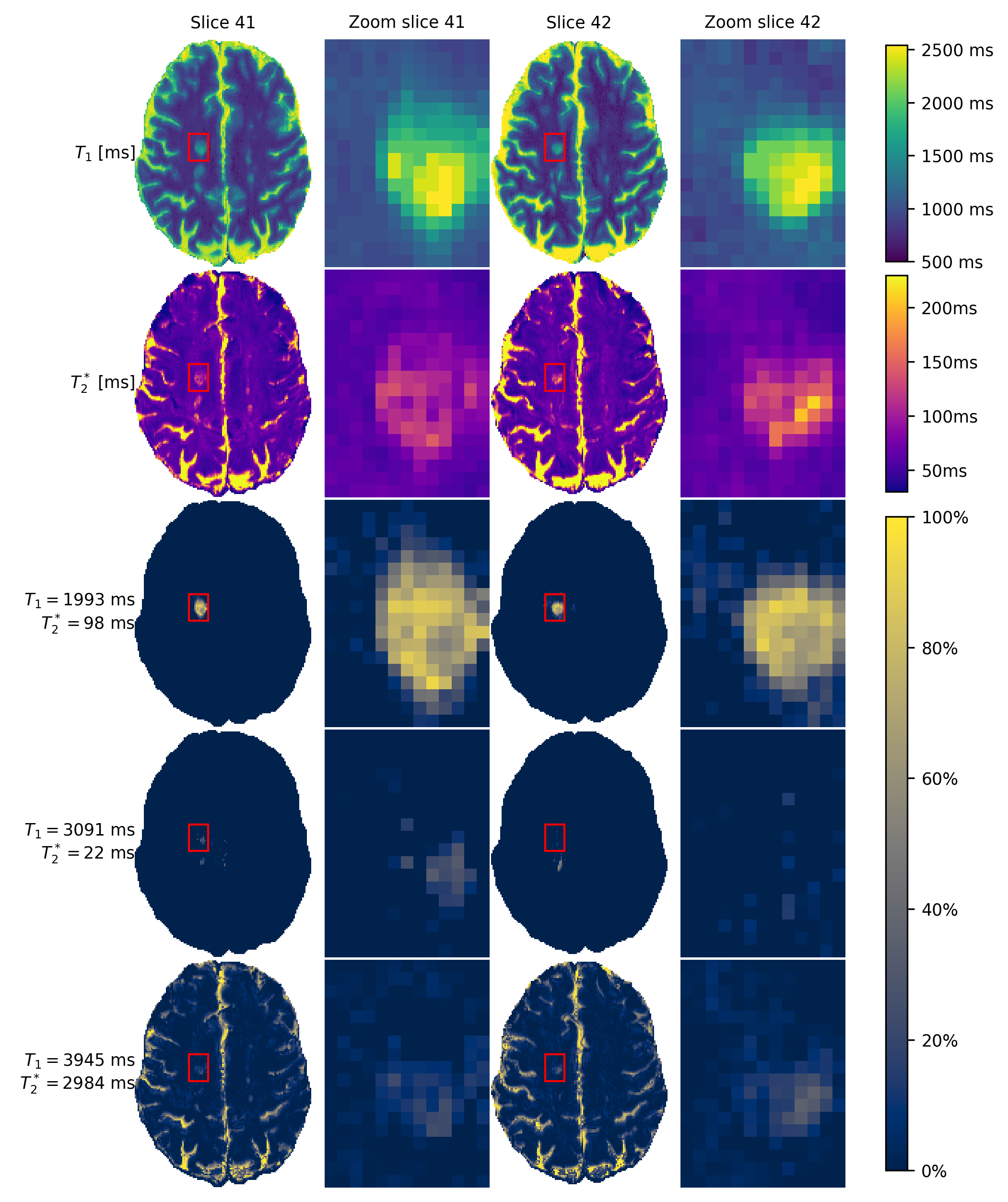
A zoomed-in version of two slices of one lesion is shown(Fig.5), including the multiple components identified in the centre of this lesion. The two detected extra components only occur with a lower fraction (~30%) and thus require multi-component sensitivity. The two components have long T₁-relaxation times, which could correspond to veins as more often observed in MS-lesions¹¹.

In this study results are shown for a single subject since the focus was on the development of the numerical methods. A topic of further research is the application to more datasets, to test the quality of the segmentations and the information contained by the smaller components in the lesions.

Conclusion

The proposed local-SPIJN algorithm is able to detect small abnormalities from MRF-EPI data. This potentially improves robustness against multi-component effects around and in lesions, paving the way for better detection and deeper insights into underlying pathological changes.

Acknowledgements

The authors would like to thank Lucas van Vliet, Dirk Poot and Thijs van Osch for their useful comments and suggestions.