Introduction

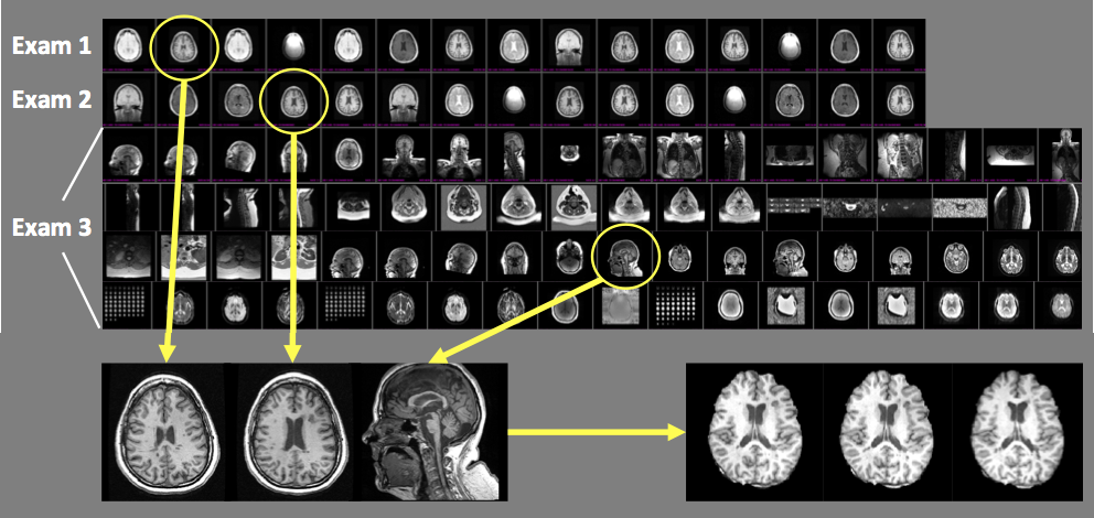
To analyze disease progression and response to therapy with MRI, it is essential to quantify serial changes that occur on images acquired with similar tissue contrast (Figure 1.) However, data in most institutional PACS systems are heterogeneous and unreliably labeled, limiting the ability to automatically retrieve and align images of the same anatomy and contrast. This problem is exacerbated in the context of processing imaging data at scale for population-level analyses. The goal of this study is to create an algorithm that can reliably retrieve images of the same contrast from a cohort of brain exams. We hypothesize that DICOM metadata features, imaging features and a combination of both should yield increasing overall, as well as per-class accuracy. We compare the contribution of radiomics imaging features and those automatically derived through CNNs, as well as model transferability within and between diseases.

Methods

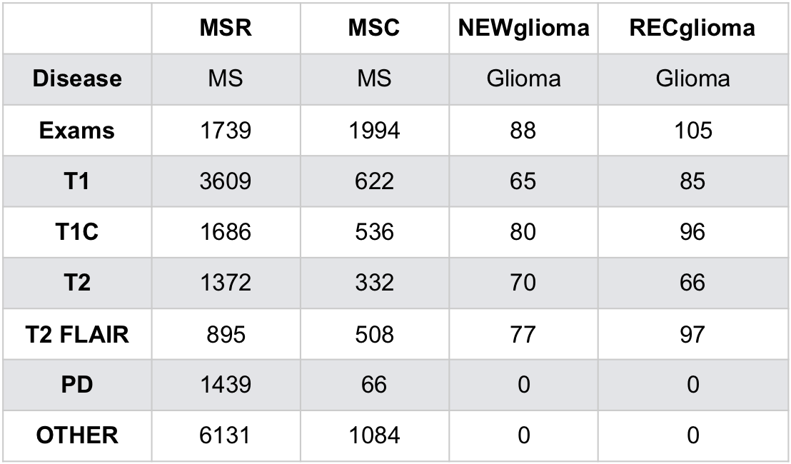
Exams and cohorts: Four cohorts (Figure 2) were used. 1) MSR, a highly uniform multiple sclerosis (MS) research cohort1; 2) MSC, a heterogeneous MS clinical cohort representative of typical, poorly labeled institutional PACS data and also representing data acquired at external sites; 3) NEWglioma and 4) RECglioma cohorts comprised of newly diagnosed and recurrent research brain tumor exams that are highly uniform in contrast and labeling. Both MSR and MSC have more uniform imaging characteristics than NEW and RECglioma which have on average much more extensive pathology per exam.
Ground truth determination: Each series used for the MSC cohort was visually reviewed and labeled; MSR, RECglioma and NEWglioma were acquired with uniform imaging protocols as part of clinical trials and already well labeled.
Training and testing splits: 1) Within-disease: training/testing splits used all of the MSR and 60% of the MSC cohort for training, while 20% MSC was used for validation and 20% was used for testing. 2) Between-diseases: training used MSR and MSC cohorts, and testing comprised all available RECglioma and NEWglioma images. In both 1) and 2), splits were randomized and stratified by outcome, with no patient leakage.
Metadata Models: Metadata were extracted from DICOM headers, hashed, and normalized to create numeric features. Series descriptions were tokenized and binarized using the top 40 most frequent words. The heuristic model was used a logical decision tree branching on a priori assumptions about acquisition parameters. SVMs were built using metadata and series descriptions features using scikit-learn’s SVC 2.
Image Processing: The center slice was used to represent each MR volume. All images normalized by subtracting the mean and dividing by the standard deviation of pixel intensity values. For radiomic analysis images were resampled to 1x1x1 mm resolution and binned into 64 intervals according to IBSI guidelines 3. All images for CNN resized to 256 x 256 pixels regardless of the FOV.
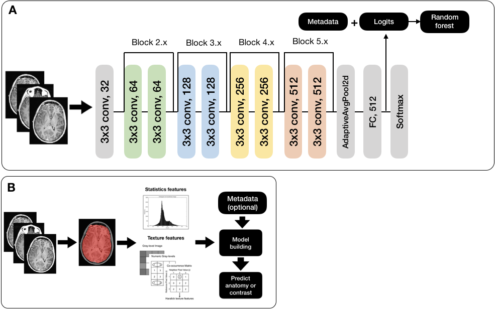
Radiomics: First and second order features were extracted using the Python pyradiomics toolkit4. SVMs were then built with the radiomics features alone and in combination with metadata features (Figure 3A).
CNN: Pre-trained ResNet-18, ResNet-34, and ResNet-505 first convolutional layers were replaced with a 1 x 64 conv layer (for grayscale DICOM images); their last layers were replaced with 512 (2048) x 6 fully connected layer (Figure 3B). A cosine differential learning rate with 3 max values (0.01, 0.001, 0.0001) was used. All model building, training, and experiments were implemented using PyTorch 1.0.0 on a Tesla V100-PCIE-32GB (NVIDIA) GPU. Metadata features were processed as described above and concatenated with logit values. A final classification was created using scikit-learn’s RFC4.

Results and Discussion

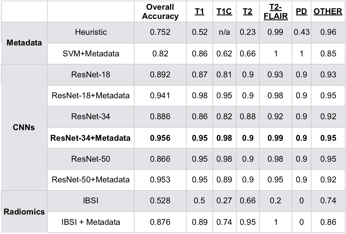
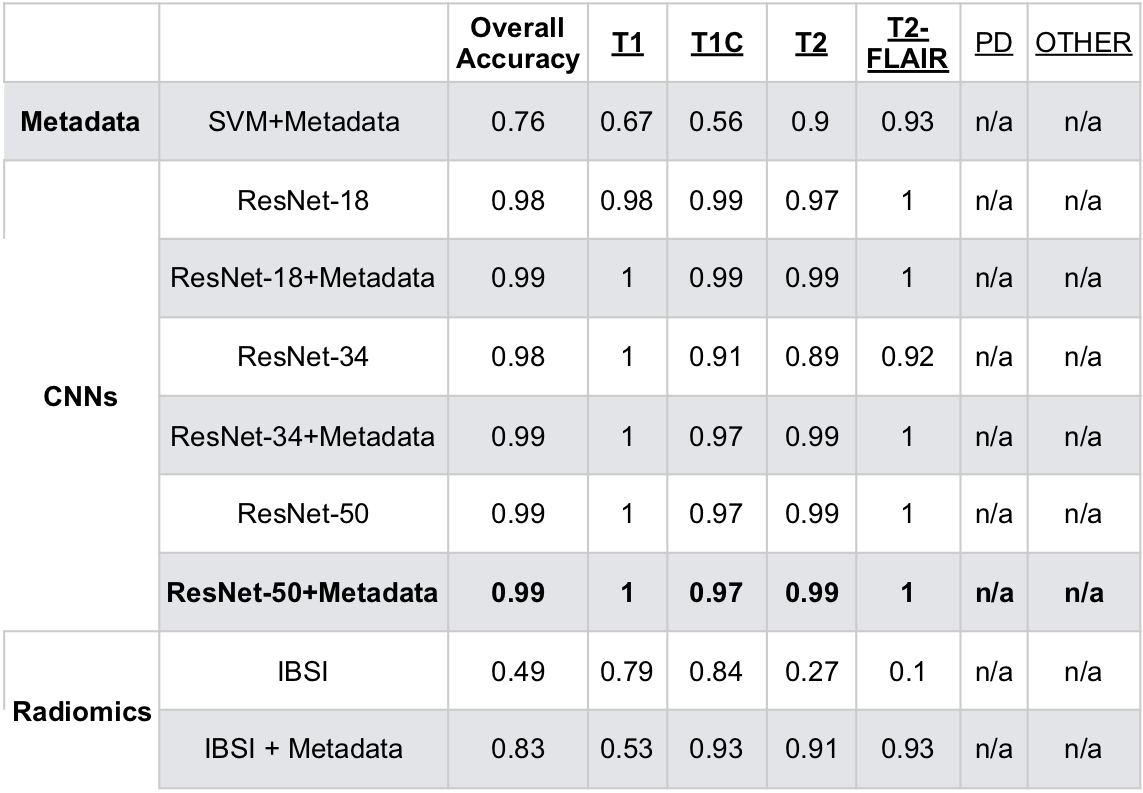
Tables 2 and 3 describe the overall accuracy and per-class accuracy for each experiment from the first (MSC) and second (glioma) train/test splits. A ResNet-34 + metadata trained on MSR + MSC and tested on MSC resulted in 95.6% overall accuracy and >95% per-class accuracy; a ResNet-50+metadata trained on MSR + MSC and tested on glioma data resulted in 99.6% accuracy >97% per-class accuracy. Taken together, these results suggest that imaging features and metadata work synergistically to represent the contrast of brain MR images. Our results comparing CNN experiments to radiomics experiments imply that the imaging features automatically generated through training a CNN are overall more valuable for classifying image contrast than standard IBSI features. Additionally, despite the distinct imaging features introduced by glioma presence, the data in RECglioma and NEWglioma were acquired with uniform imaging protocols compared with the MSC cohort which could explain why our between-disease results are Additionally, manually labeling the MSC dataset is imperfect and introduces some error into the ground truth labels, whereas the labels of the other cohorts were derived from rigid clinical trial protocols. Next, we plan to expand this to more contrast types (e.g. diffusion, perfusion) and test on a cohort from a different disease from a different institution.

Conclusion

In this study, we compare the results of using DICOM metadata, IBSI radiomics imaging features, and CNN imaging features to classify the contrast of brain MRI images. We conclude that for both within-disease and between-disease prediction, deep ResNets for imaging feature extraction combined in a random forest with DICOM metadata performs best and can be deployed to reliably deliver images of specific contrasts for clinical use or large imaging analyses.

Acknowledgements

No acknowledgement found.