INTRODUCTION
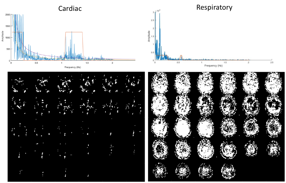
In the recent years, there has been increasing interest in assessing the extent of resting-state connectivity at frequencies higher than traditionally used (> 0.15 Hz).^1-4 The existence of statistically significant correlations in the high frequency range (> 0.15 Hz) would inform modeling of neurovascular coupling mechanisms and may improve characterization of resting state networks. However, characterizing the extent of these networks remains a challenge as much of the high frequency information is inaccessible due to confounding physiological pulsation. While physiological noise due to respiration is present in much of the brain as shown in Figure 1, cardiac noise is much more localized. Therefore, the use of global frequency filters may remove neuronal information from regions where cardiac contamination is weak. Spatially selective filters, however, necessitate the development of new model-based detection algorithms that could dynamically identify and filter physiological noise from the data.
METHODS
An in-house MATLAB based toolbox, TurboFilt, was developed for the processing and filtering of fMRI data. A key functionality in the toolbox is the automated filtering capability which can automatically detect and filter physiological noise through the following steps:
(a) Physiological noise detection The program uses a clustering algorithm in the spectral domain combined with power law fitting of the spectral data to identify physiological confounds in the frequency domain. The purpose of the clustering step is to allow for the detection of spectral confounds with complex shapes such as those with fluctuating patterns and also to reduce the number of filter bands applied in such situations. For optimal processing and for consistent filtering, the detection process is done in spatial kernels. The spatial data is coarsified by dividing the domain into kernels of equal sizes. Kernels may alternatively be explicitly specified through the use of masks. This allows for physiologically informed detection but requires additional information to be supplied.
(b) Frequency filtering Zero-phase FIR filtering with order < sample size/3 is done at the voxel level relying on detections at the kernel level. The voxels that fall under each kernel are filtered based on the detected spectral confounds for the kernel. In the case of mask-defined kernels, a voxel may fall under no kernel at all. In that case, the signal in the voxel is filtered using the combined detections from all other kernels. The filter application may be restricted to an arbitrary frequency range supplied by the user.
(c) Temporal PCA Regression of physiological noise, for example as described by Gembris et al. (2000), is effective at removing low frequency contamination.⁵ In the present protocol, a temporal PCA is used in order to identify respiratory components and low frequency contaminants (e.g. motion components) in the data analogous to Behzadi et al (2007).⁶ The PCA components are obtained from voxels with 95th percentile standard deviation in signal intensity. The five PCA components with most variability are used as regression vectors to remove low frequency confounds from the data.
Seed-based correlation analysis over the entire time domain is used to probe the connectivity networks and the effectiveness of the algorithm in cleaning up the data.
RESULTS AND DISCUSSION
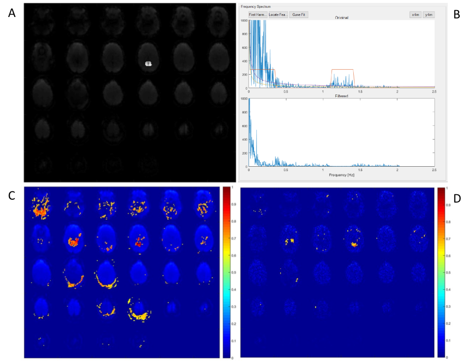
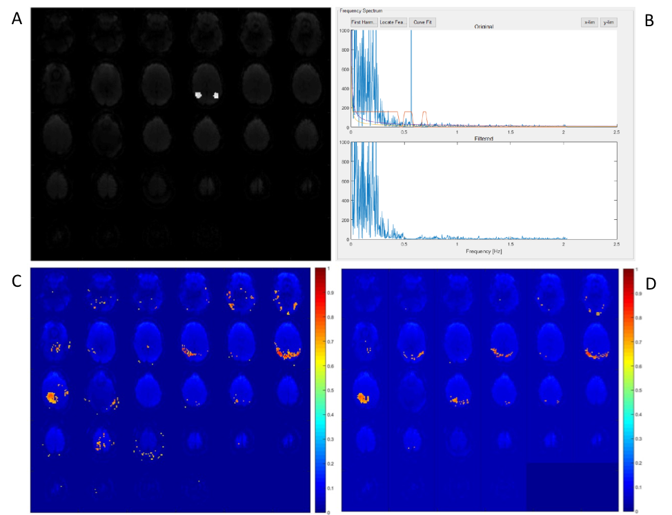
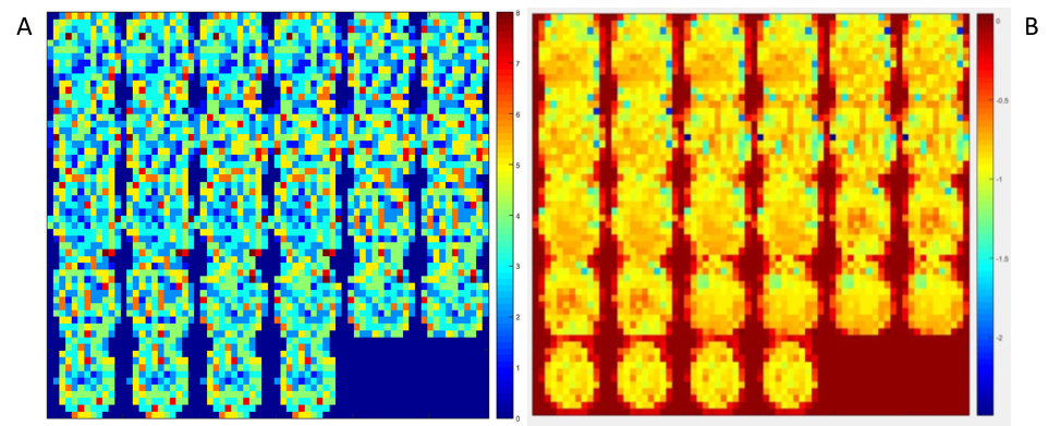
Preliminary application of the approach has been conducted with the intent to assess the ability of the algorithm to detect and filter spectral confounds. Figures 2 and 3 demonstrate examples of this preliminary application. The scan in these examples used a TR of 0.246 seconds which enables aliasing-free sampling up to 2 Hz. In the case in Figure 2, filtering is applied to spectral confound detections in the entire spectral range, while in Figure 3 it’s restricted to detections after 0.5 Hz as shown in Figures 2.B and 3.B. Spatial kernels of 4x4x4 voxels are used for the detection in both cases. In Figure 2, a significant reduction in artifactual connectivity is observed compared to the case with no filtering. In Figure 3, similar results are observed. However, in both cases some artifactual connectivity remains. This may be attributed to imperfections in the detection of isolated frequency confounds with narrow bands. Figure 4.A shows the number of filters applied in each voxel for the case in Figure 2. The mean number of filters applied per voxel was ~3. However, in some voxels, as many as 8 filters were applied. This is a result of using a constant spectral cluster size criterion for all voxels. This may be remedied by using an iterative feedback loop based approach which could adjust the cluster size criterion locally based on the number of filters applied in the previous iteration in the kernel. Additionally, Figure 4.B shows the distribution of the exponent obtained from the power law fit in the spectral domain. It can be observed that the exponents near the edges and near the center of the brain are relatively weaker in magnitude which suggests regional dependence of the fit. The use of kernels reduced processing time from ~5 hours to ~7 min on 20 cores of Intel Xeon E5-2697 v4. Such a tool may be useful in characterizing the spatial dependence of the hemodynamic response function assuming that the data is cleaned of physiological confounds which can influence the fits.

Acknowledgements

This research was supported by 1R21EB022803-01. We gratefully acknowledge Victoria Bixler and Amanda Gurule for their assistance with MR operations. Special thanks to our research participants.