1518
In-vivo Visualization of Locus Coeruleus using MTC-STAGE Imaging1Radiology, Ruijin Hospital, Shanghai Jiao Tong University School of Medicine, Shanghai, China, 2Radiology, Changshu Hospital Affiliated to Nanjing University of Chinese Medicine, Changshu, China, 3Neurology, Wayne State University, Detroit, MI, United States, 4Philips Healthcare, Shanghai, China, 5Radiology, Wayne State University, Detroit, MI, United States, 6Biomedical Engineering, Wayne State University, Detroit, MI, United States
Synopsis
The locus coeruleus (LC) is mainly responsible for the synthesis of noradrenaline in the brain. Pathological alterations of the LC are involved in many neurodegenerative diseases. In this work, we use the tissue properties (spin density and T1 value) of the LC extracted from an MTC-STAGE (strategically acquired gradient echo) susceptibility weighted imaging protocol. Choosing the right flip angle and resolution can provide optimal visualization of the LC. We found that a short echo scan, with a flip angle of 25-30o and a resolution of 0.67 x 0.67 x 1.34mm3 provides the best visualization of the LC.
Introduction
The locus coeruleus (LC) is a neuromelanin-rich structure and located in the dorsal part of the pons in the brainstem. It is the main source of noradrenaline in the brain. The LC has been identified as the major site of subcortical neuronal loss in both Parkinson’s disease (PD) and Alzheimer’s disease1. Imaging the LC holds promise for detecting early stage degeneration in PD patients and may help to facilitate the application of timely symptomatic interventions2. Magnetization transfer contrast (MTC) imaging has been used to visualize neuromelanin (NM) predominantly due to the suppression of surrounding tissues while leaving the LC otherwise visible3. It is believed that the LC can be depicted because of the T1 weighting (T1W) and high flip angles used. However, bright tissue in an MTC image usually means high water content since otherwise the signal will be significantly suppressed. The aim of this study is to optimize the imaging protocol from the perspective of flip angle and resolution by measuring the tissue properties (spin density and T1 value) of the LC using MTC-STAGE (strategically acquired gradient echo)4-6 susceptibility weighted imaging (SWI).Methods
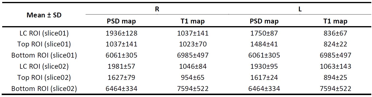
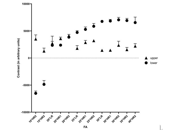
A total of 3 healthy volunteers (ages 20, 20, 23 years old) were scanned on a 3T Philips MRI system with a 15-channel coil using a 3D multi-echo gradient echo SWI sequence with an MTC pulse. The imaging parameters were as follows: seven echoes with TE1 = 7.5ms, ΔTE = 7.5ms, with TR = 62ms, pixel bandwidth = 174Hz/pixel, matrix size = 384 × 384, slice thickness = 2mm. For each acquisition, the field-of-view was placed perpendicular to the fourth ventricle and parallel to the anterior commissure-posterior commissure line. In order to extract the tissue properties, we collected the data with multiple flip angles ranging from 10o, 15o, 20o, 25o, 30o, 35oand 40o with three different resolutions: low resolution (LR) (0.67×1.34×2 mm3), high resolution 1 (HR1) (0.67×0.67×2 mm3) and HR2 (0.67×0.67×1.34 mm3). Thanks to collecting many flip angles (FA) high quality T1maps and spin density maps can be obtained from the MTC-STAGE reconstruction. We utilized the shortest echo (TE=7.5ms) in the MTC-SWI magnitude image to depict the NM content in LC. The contrast of the LC compared to surrounding tissues is defined as: contrast = SLC –Sref where SLC is the mean signal intensity of the LC and Sref is the mean signal intensity of the reference region. We chose the adjacent grey matter (above the LC) and the fourth ventricle (below the LC) as our reference regions.Results
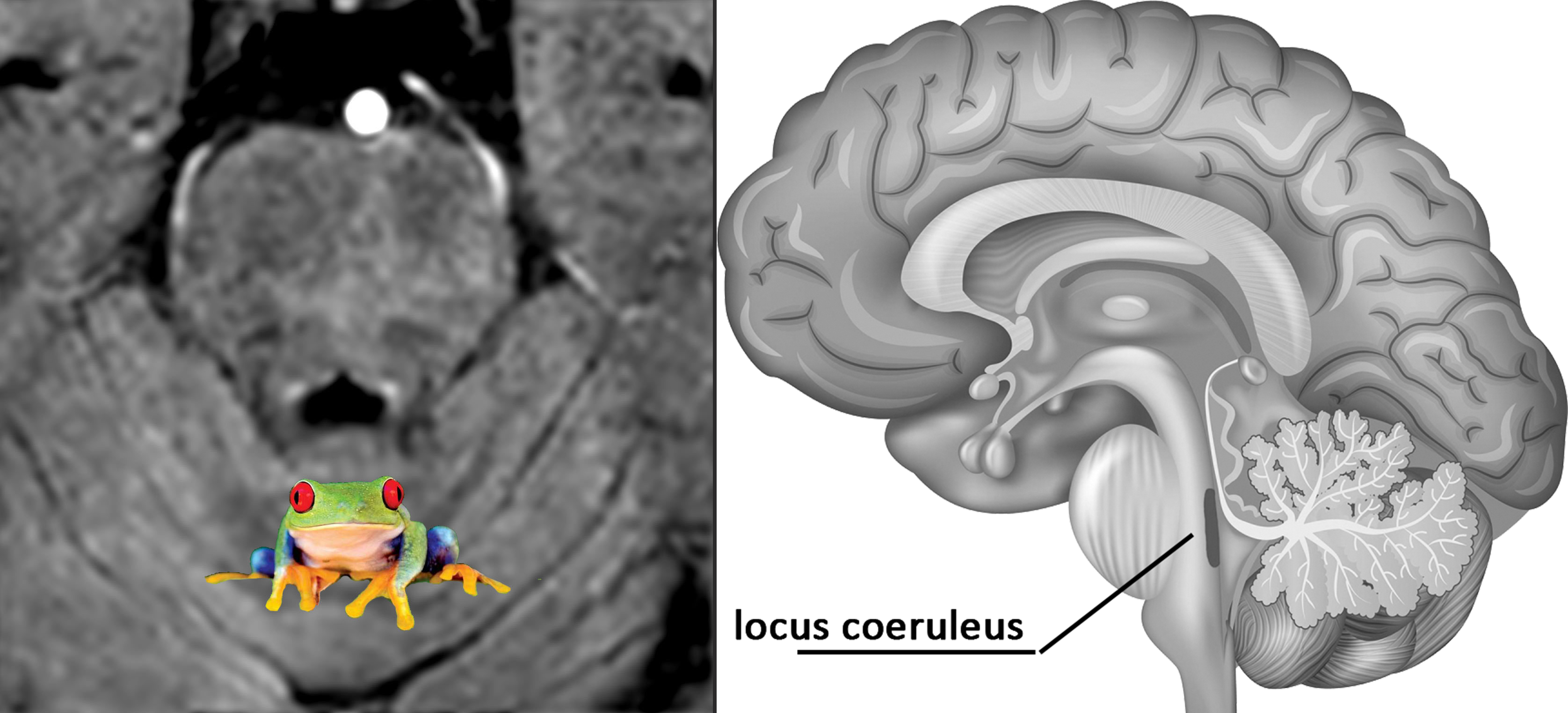
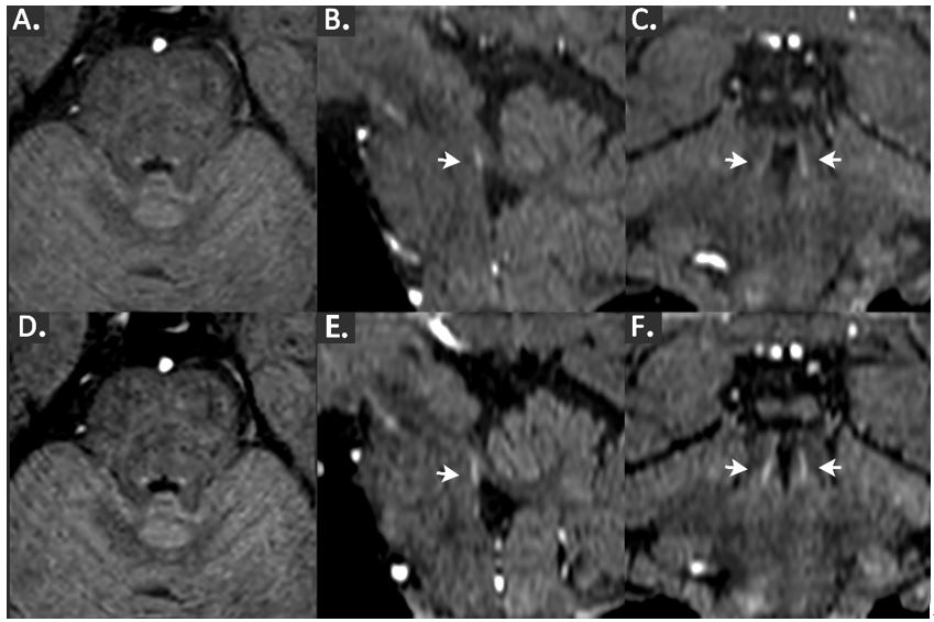
Figure 1 shows two bright circular hyperintensities anterior to the fourth ventricle which corresponded to the shape and anatomical locations of the right and left LC. These two high intensity signals remind one of symmetric frog eyes (see inset into Figure 1). Once we chose the proper imaging parameters, these frog eyes light up. Figure 2 shows images with different FAs and resolutions. Owing to the two different reference regions above and below the LC, we see that the LC “frog eyes” appear brightest and most well defined for the 25oand 30o FA images with a resolution of 0.67×0.67×1.34 mm3. To understand this contrast behavior, we measured the spin density and T1 values from the STAGE data (Table 1). The T1 value of the LC is on the order of 1000ms while the tissue above is roughly the same.Discussion and conclusion
Recent advances in measuring tissue properties with methods like STAGE facilitate in-vivo assessment of the LC. Optimizing its contrast to noise allows for the best choice of resolution in a practical imaging time of 7 minutes in this study. By understanding the tissue properties of the LC, we can best optimize the imaging parameters where we found that 25o or 30o did the best job. After the MT pulse is applied, the effective T1 values of all tissues is reduced, more so for those with low water content and high macromolecular content (like white matter). While those tissues with higher water content are not suppressed as much. However, in this case the two tissues (LC and top region) have similar T1 values but the LC has higher water content. Therefore, one would expect a flip angle that is near the Ernst angle to provide the best contrast (otherwise the contrast-to-noise (CNR) will reduce if too large a flip angle is used). From a resolution perspective, the best CNR for a small structure can occur for the high resolution scans since otherwise significant blurring will occur. The in-plane resolution of isotropic 0.67mm made a big difference in LC visibility. In the same way, if the LC is angle in the coronal view a thinner slice should likewise improve visibility. We found that a 1.34mm slice was a good compromise to better visualize the LC coronally. As LC imaging is thought to also be affected in dementia and more recently NM content has been suggested to correlate with the clinical status of PD7. Therefore, the best visualization that can be obtained at 3T is critical if this is to become a practical imaging protocol.Acknowledgements
No acknowledgement found.References
1. Chris Zarow et al. Neuronal loss is greater in Locus Coeruleus than Nucleus Basalis and Substantia Nigra in Alzheimer and Parkinson diseases. Arch Neurol 2003;60:337-341
2. Matthew J. Betts et al. Locus coeruleus imaging as a biomarker for noradrenergic dysfunction in neurodegenerative diseases.BRAIN 2019; 0:1–14
3. Priovoulos Net al.High-resolution in vivo imaging of human locus coeruleus by magnetization transfer MRI at 3T and 7T. NeuroImage2018;168:427-436.
4. Chen Y, Liu S, Wang Y, Kang Y, Haacke EM. STrategically Acquired Gradient Echo (STAGE) imaging, part I: Creating enhanced T1 contrast and standardized susceptibility weighted imaging and quantitative susceptibility mapping. Magnetic resonance imaging 2018;46:130-139.
5. Wang Y, Chen Y, Wu D, et al. STrategically Acquired Gradient Echo (STAGE) imaging, part II: Correcting for RF inhomogeneities in estimating T1 and proton density. Magnetic resonance imaging 2018;46:140-150.
6. Haacke EM, Chen Y, Utrainen D, et al. STrategically Acquired Gradient Echo (STAGE) Imaging, part III: Technical Advances and Clinical Applications of A Rapid Multi-Contrast Multi-Parametric Brain Imaging Method. Magnetic Resoannce Imaging 2019;DOI:10.1016/j.mri.2019.09.006.
7. Sulzer Det al. Neuromelanin detection by magnetic resonance imaging (MRI) and its promise as a biomarker for Parkinson's disease.NPJ Parkinsons Dis. 2018; 4: 11
Figures