1429
A novel multicomponent T2 analysis for identification of sub-voxel compartments and quantification of myelin water fraction1Department of Biomedical Engineering, Tel Aviv University, Tel Aviv, Israel, 2Department of Computer Science and Applied Mathematics, Weizmann Institute of Science, Rehovot, Israel, 3Center for Advanced Imaging Innovation and Research (CAI2R), New-York University Langone Medical Center, New York, New York, NY, United States, 4Sagol School of Neuroscience, Tel-Aviv University, Tel Aviv, Israel
Synopsis
Multicomponent T2 analysis (mcT2) can be highly valuable for probing tissue microstructure. However, it remains challenging due to its ill-conditioned nature, and due to inherent contamination of multi spin-echo signals by stimulated echoes. We present a novel mcT2 algorithm that tackles the high-dimensionality of this problem, using correlations between local and global features of the anatomy in question. The accuracy of this tool is demonstrated on phantoms and in vivo. Our results suggest that the method can accurately identify microscopic compartments, operate at realistic scan times, and be used estimate to estimate myelin content in vivo.
Introduction
The assessment of myelin content in white matter (WM) provides valuable information regarding neurodegenerative diseases, as well as insights on neuronal maturation and development1,2–5. Myelin water fraction (MWF) is a proxy for myelin content, which can be estimated using multicomponent analysis of T2 relaxation times (mcT2). This estimation is done through a fitting process where a weighted sum of different T2 components (i.e. spectra) is matched to multi-echo spin-echo (MESE) signal decay curve. However, the detection of the true T2 distribution is a highly ill-posed problem6,7, especially at low-to-moderate signal-to-noise ratios (SNRs)8. In this study we present a new approach to mcT2 analysis from MESE signals. To overcome the problem’s non-uniqueness we generate a dictionary of possible T2 distributions of different tissue types, and exploit correlation between local and global features to choose a small set of basis-functions for the fitting process. The algorithm can be applied to clinical MESE data and the resultant spectra can be further analyzed to identify different tissue microenvironments, as well as, to quantify MWF.Methods
Fitting algorithmThe proposed signal-deconvolution algorithm begins with fitting a single T2 to each MESE signal. To compensate for the non-exponential signal decay due to stimulated and indirect echoes10 we employ the echo modulation curve (EMC) algorithm. This technique was previously shown to produce accurate and reproducible T2 values11, by accounting for specific protocol implementation, hardware imperfections, and scan parameters to form a simulated MESE signal. Next, we used the same model to simulate a series of multi-T2 signals each containing 1-3 components with relative fractions between 0.1-1: $${S_{mc}= \sum_{i=1}^3w_i\cdot S_{T_{2}}}, s.t. \sum_1^3w_{i} = 1$$ where: $$$S_{T_{2}}$$$ is the MESE relaxation pattern for the ith T2, $$$w_i$$$ is the relative fraction of the T2 component, and $$$S_{mc}$$$ is the simulated multicomponent-MESE signal. Next, a score is calculated for each simulated signal based on its L2-norm correlation to each of the pixels in the segment of interest. These scores are summed up, producing a global similarity score for each simulated multi-T2 signal. Lastly, we choose the 50 multi-T2 signal options with the highest score and consider those basis-function for the subsequent optimization process. The problem is defined as a quadratic least-squares6 and a quadratic programming solver with L1 regularization term is applied on the set for the fitting task.
Validation
Numeric simulation: A 2D Shepp–Logan numerical phantom was generated, consisting of 5 tissue types (Fig. 1). Each type reflected a different distribution of three T2 components (detailed in Fig. 1) with varying fractions (detailed in Fig. 2). The MESE signal from each compartment was simulated using a weighted-sum of the components at each pixels in the phantom. To simulate realistic condition, Gaussian noise, and natural variation of 20% in T2 values were added to the signals prior to analysis.
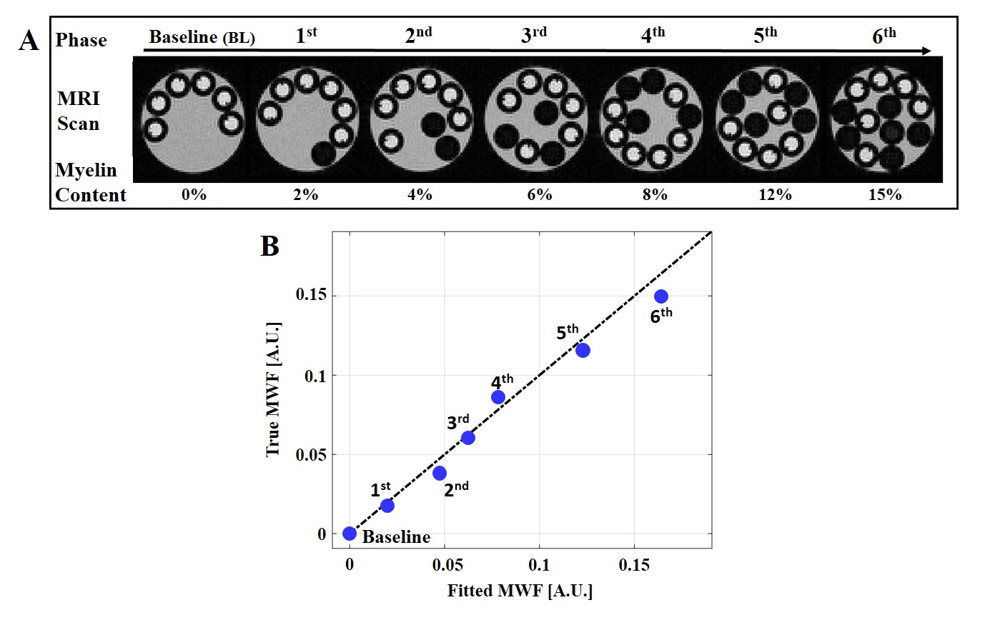
Phantom scans: A unique multi-compartment T2 phantom was prepared from 3 MnCl2 solutions inducing different T2 values. A 50ms solution was filled within a 5mm tube with a varying number of 1mm tubes filled with T2={13 and 80ms}. Smaller tubes were consecutively inserted between scans into the 5mm tube. The phantom was scanned 7 times on a Bruker,9.4T scanner with a different number of small tubes inducing varying fractions. This phantom’s design allowed us to map high-resolution T2 values in all three environments and to perform a low resolution scan where all three compartments occupied a single pixel. Low resolution data was deconvolved using our mcT2 algorithm and the resulting T2 spectra validated against ground-truth values. To estimate MWF, the area under the short T2 component were calculated from the resultant T2 spectra12.
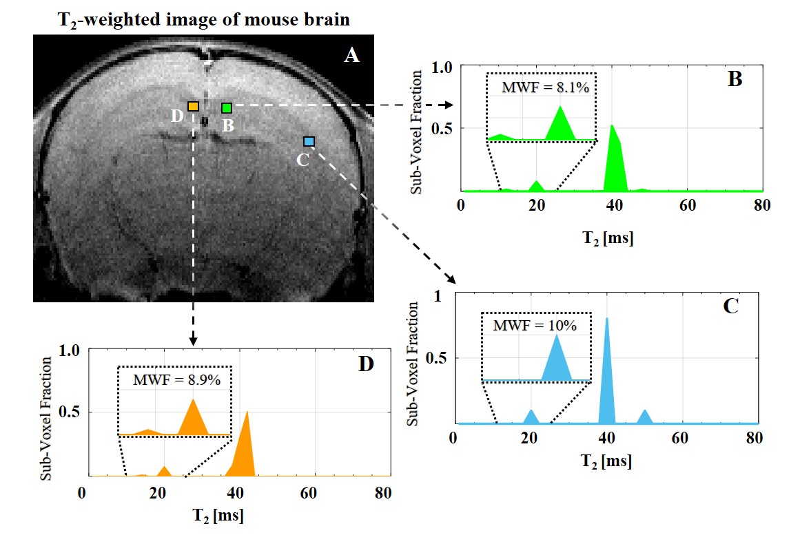
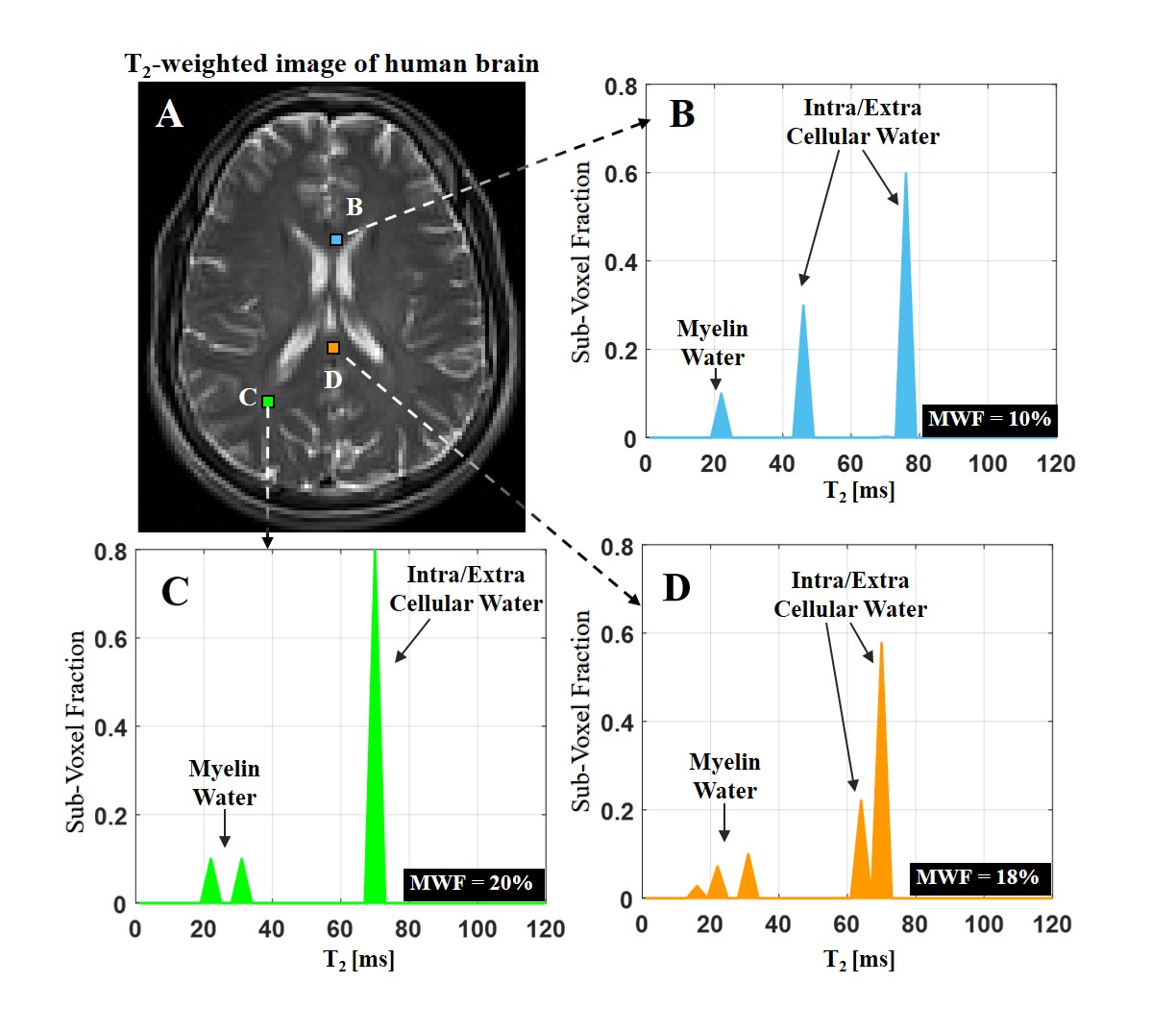
In vivo: MESE brain data (30 echoes and 2 averages) were acquired from healthy mouse (Bruker, 7T) and human volunteer (Siemens, 3T). T2 spectra were fitted to all voxels and MWF were estimated in selected WM pixels.
Results
T2 spectra of numerical phantom were perfectly reconstructed with 1, 2 and 3 compartments respectively, and at SNR level of 60 and above (Fig. 2). Fig. 3 presents the goodness-of-fit for the phantom, demonstrating high accuracy between calculated and actual MWF (p<0.01, R-square=0.98). Applying the algorithm on in vivo mouse and human data produced the T2 spectra seen in Fig. 4-5, having 2 and 3 distinct compartments and T2 values and fractions within physiological range2: T2 mouse: {20ms, 40ms 50ms} and T2 human: {20ms 50ms 78ms}. Although no ground truth was available for this data, the estimated MWF at 3 different locations were consistent with literature12,13: mouse {8%, 8.9%,10%}, and human {10%, 18%, 20%}.Discussion and Conclusion
Presented results attest to our mcT2 algorithm’s ability to probe distinct sub-voxel compartments at realistic scan conditions. The excellent agreement shown for the MWF phantom suggests that the method has the potential to accurately quantify myelin content. The presented algorithm has three notable advantages: first, it learns the anatomy prior to analyzing each specific voxel; secondly, it does not impose prior distribution of T2 values; and third, and most importantly, it does not use a predefined fixed number of components, but rather manages to accurately identify this number based on the acquired data. Further validations are now begin conducted, comparing MWF values to ground-truth myelin content extracted from histology.Acknowledgements
ISF Grant 2009/17References
1. Heath F, Hurley A, et al. Advances in noninvasive myelin imaging. Dev. Neurobiol. 2018;78:136–151.
2. Zhang, J, Kolind S, et al. Comparison of Myelin Water Fraction Brain Images Using Multi-Echo T2-Weighted GRASE Relaxation and Steady-State Methods. Proc Intl Soc Mag Reson Med. 2015;73(1):1025-1029.
3. McCreary R, et al. Multiexponential T2 and magnetization transfer MRI of demyelination and remyelination in murine spinal cord. Neuroimage. 2009;45(4):1173-1182.
4. Möller E, et al. Iron , Myelin , and the Brain : Neuroimaging Meets Neurobiology. Trends Neurosci. 2019;42(6):384-401.
5. Alonso-Ortiz E, Levesque R, et al. MRI-based myelin water imaging: A technical review. Magn. Reson. Med. 2015;73(1):70-81.
6. Whittall P and MacKay L. Quantitative interpretation of NMR relaxation data. J. Magn. Reson. 1989;84:134-152.
7. Laule C, et al. Water content and myelin water fraction in multiple sclerosis - a T2 relaxation study. J. Neurol. 2004;251:284–293.
8. Whittall P, et al. In vivo measurement of T2 distributions and water contents in normal human brain. Magn. Reson. Med. 1997;37:34–43.
9. Bouhrara M, Spencer G. Improved determination of the myelin water fraction in human brain using magnetic resonance imaging through Bayesian analysis of mcDESPOT. Neuroimage. 2019;127:456–471.
10. Hennig J. Multiecho imaging sequences with low refocusing flip angles. J Magn Reson 1988;78:397–407.
11. Ben-eliezer N, Sodickson D K, et al. Rapid and Accurate T2 Mapping from Multi–Spin-Echo Data Using Bloch-Simulation-Based Reconstruction. 2015;73(2):809-817. 12. MacKay L, Laule C. Magnetic Resonance of Myelin Water: An in vivo Marker for Myelin. Brain Plast. 2016;2:71–91.
13. Kathryn W, Nathaniel K, et al. Myelin water fraction imaging with MRI. NeuroImage 2018;2:511–521.
Figures
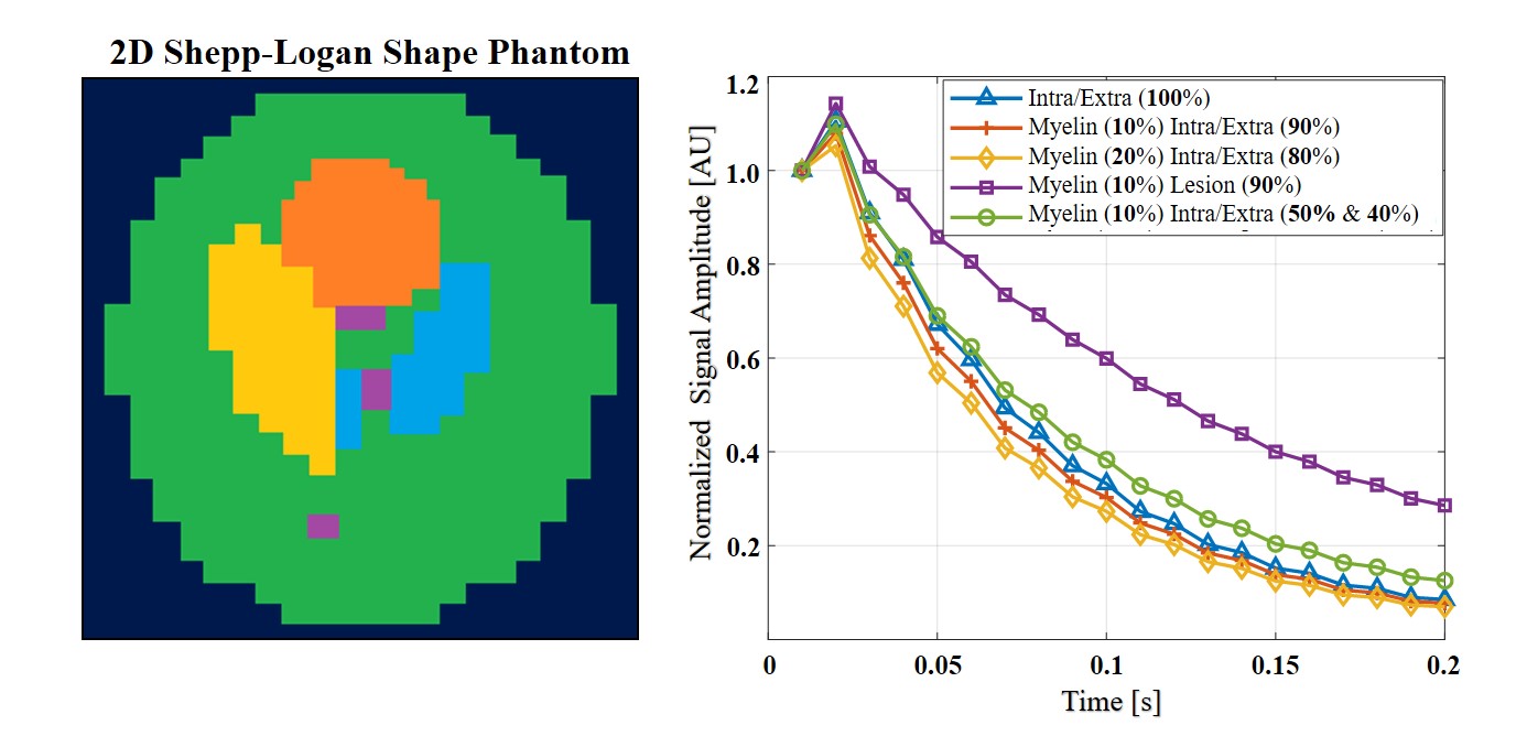
Figure 1: (Left) A 2D display of the Shepp-Loagn phantom presenting the five different tissue microenvironments with different colors. (Right) Normalized simulated MESE signals. Prior to the reconstruction Gaussian noise was added to the signals (SNR 60) and random T2 values, ranging between 20% from the true T2 values were simulated within the segments.
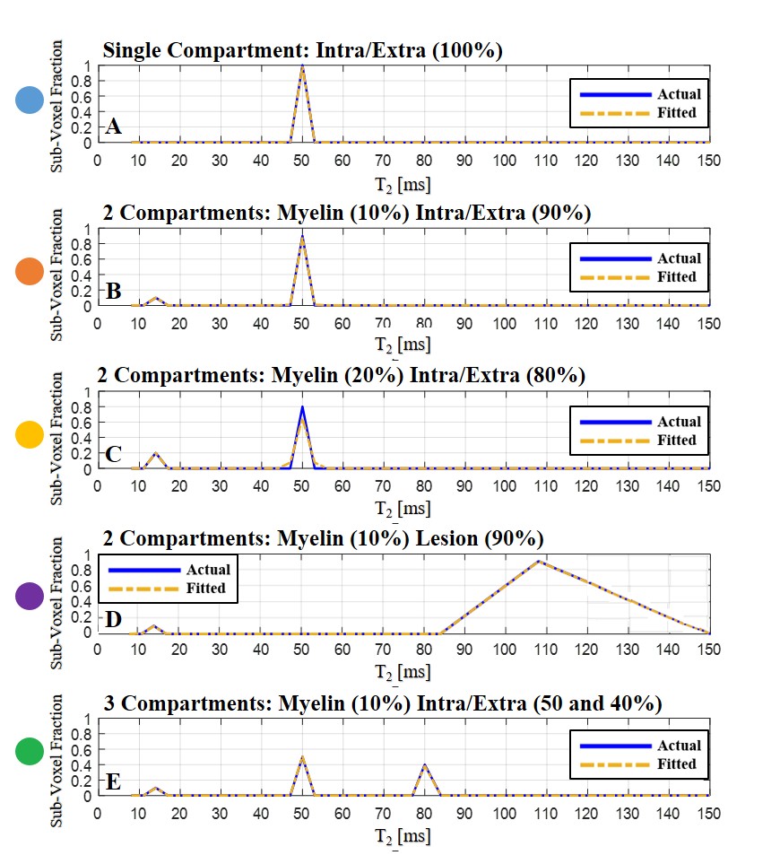
Figure 2: (A-E) A successful reconstruction of T2 distributions (dotted orange line) vs. the actual spectra (continuous blue line) from noisy simulated MESE signals (SNR 60). T2 distributions are marked with matching segment colors as indicated Fig. 1.