1428
Model-based T2* autoencoder for Myelin Water Fraction Mapping1Electrical and Electronic Engineering, Yonsei University, Seoul, Republic of Korea
Synopsis
In this study, we propose a model-based unsupervised learning algorithm to estimate three-component exponential model parameters. The proposed method, model-based T2* autoencoder, is composed of ANN encoder and three-component model decoder. Incorporation of ANN encoder and three-component model decoder provides noise robust estimation of MWF and physically meaningful information at deep latent space.
Introduction
Myelin Water Fraction (MWF) mapping is a quantitative imaging technique to investigate the water trapped between myelin lipid bilayers [1-2]. As a T2* based MWF mapping, multi-echo gradient recalled echo (mGRE) has been explored by using three-component exponential model [3-5]. The model parameters are estimated by non-linear curve-fitting algorithm. Due to ill-posedness of fitting multi-exponential model, curve-fitting algorithm requires strict constraint for initial/upper/lower values and high SNR. An artificial neural network (ANN) has been implemented to T2 based MWF mapping and demonstrated noise robustness [6]. However, the ambiguity of true value of three-component T2* sources makes it difficult to apply ANN to MWF mapping. Recently, as an unsupervised learning approach, convolutional neural network encoder and model decoder (CEMD) has been suggested in 1H spectral fitting [7]. In typical autoencoder which consists of ANN encoder and ANN decoder, the training is processed to reconstruct the input signal by minimizing the error of input and output signal [8]. In this study, we propose a model-based T2* autoencoder for unsupervised learning of model parameters. By incorporating three-component exponential model decoder, the latent space can represent the physically meaningful parameters that could not be interpreted in typical machine leaning approach. The proposed method shows noise robustness and independence of initial/upper/lower values.Method
[Conventional curve-fitting algorithm for GRE-MWI]The three-component complex model fits the decay curve to the following:
$$s(t) = (A_{my}e^{-(1/T_2,my^*+i2\pi\triangle f_{bg+ax})}+A_{ax}e^{-(1/T_2,ax^*+i2\pi\triangle f_{bg+ex})}+A_{ex}e^{-(1/T_2,ex^*+i2\pi\triangle f_{bg+ex})})e^{-i\phi_{0}}$$
where $$$A_{my}, A_{ax}$$$ and $$$A_{ex}$$$ are the amplitude of the three water components, $$$T_2,my^*, T_2,ax^*$$$ and $$$T_2,ex^*$$$ are T2* of three water components, $$$\triangle f_{bg+my}, \triangle f_{bg+ax}$$$ and $$$\triangle f_{bg+ex}$$$ are sum of frequency offset of each pool and the background. The fitting parameters are estimated by solving an iterative nonlinear least squares curve-fitting [3-5]. The initial values and upper/lower bound values were set the same as in [8].
[Training of model-based T2* autoencoder]
The proposed autoencoder is consist of ANN encoder and model-based decoder (Fig. 1).
In ANN encoder, the dimension of input signal is reduced to the model parameters as: $$f_{E}:R^{N_{t}}\rightarrow R^{N_{p}}, f_{E}(s,W) = \theta$$ where $$$f_{E}$$$ is encoder which consists of fully-connected (FC) layers, $$$s(t)$$$ is input signal, $$$\theta$$$ is model parameters, W is weights of FC layers. $$$N_{t}$$$ and $$$N_{p}$$$ are the size of input signal and the model parameters respectively.
In model-based decoder, the model parameters are mapped to output signal by using three-component complex model as:
$$f_{D}:R^{N_{p}}\rightarrow R^{N_{t}}, f_{D}(\theta) = \widehat{s}
$$ where $$$f_{D}$$$ is decoder which consists of three-component complex model, $$$widehat{s}$$$ is output signal. Finally, the objective function for training is as:
$$\lim_{W}[f_{D}(f_{E}(s,W))-s]$$
The training data are adopted from mGRE signal in entire brain region except skull by using FSL software. The number of voxel-wise mGRE signal for training is ~100,000 for a single subject.
After learning the weights of the autoencoder layers, the mGRE signal is put into the autoencoder in voxel by voxel. By investigating the deepest latent space, model parameters ($$$\theta$$$) of each voxel are estimated.
[Data Acquisition]
Data from a healthy volunteer was acquired on a clinical 3 Tesla MRI scanner (Tim Trio, Siemens Medical Solution, Erlangen, Germany) using a 12-channel head coil. The 3D mGRE data were acquired as followed: FOV = 256x256x144mm3, spatial resolution = 2x2x2mm , flip angle = 20°, TR = 60ms, TE1 = 1.6ms, ΔTE = 1.1ms, # of echoes = 30. Additionally, MPRAGE was acquired for anatomical reference.
Result
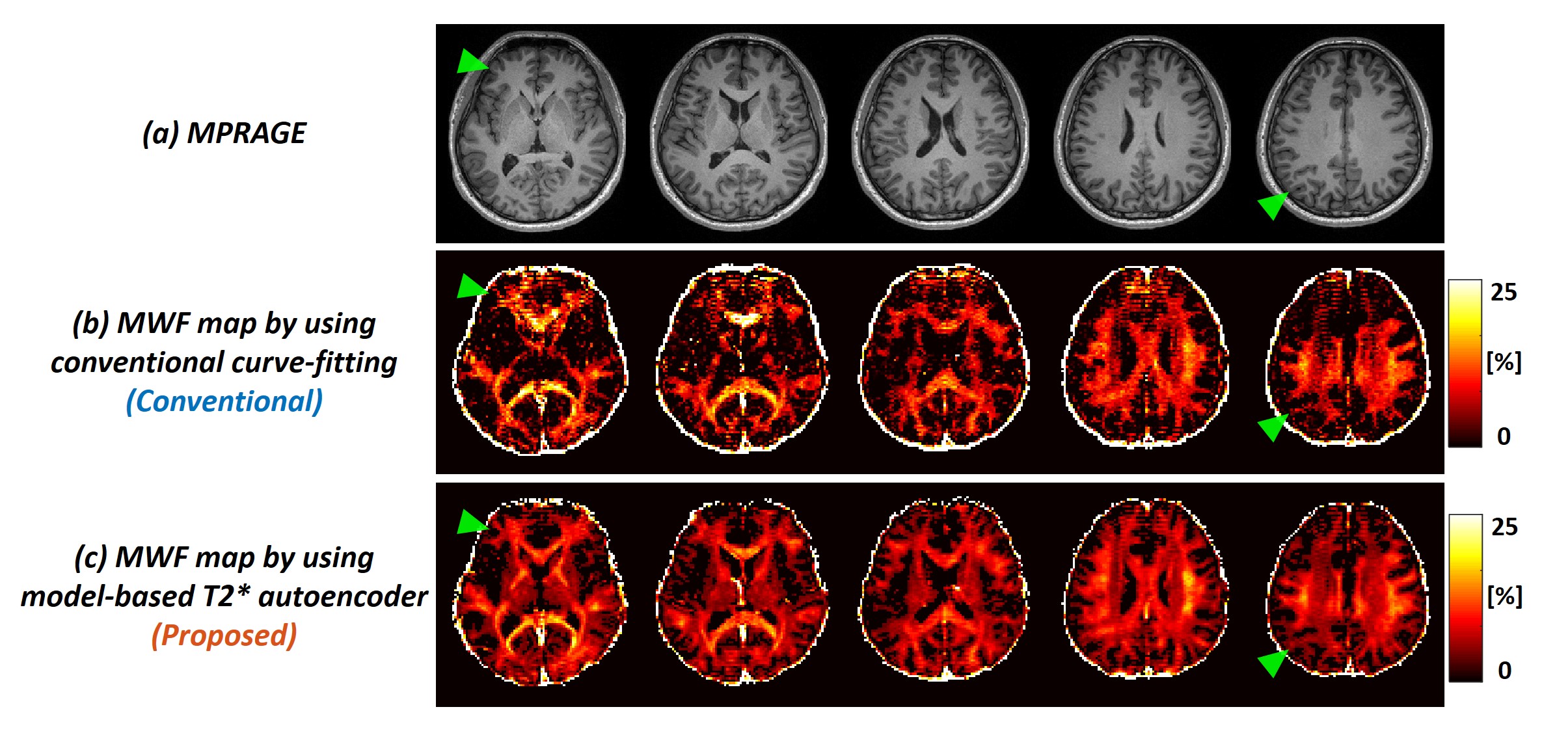
Figure 2 shows the histogram of model parameters for white matter region. The estimated amplitude of axonal/extracellular water from proposed method represented decreased variation compared to conventional method. The estimated T2* from conventional method represented bias to initial guess and upper bound (red arrow in Fig. 2b). The estimated T2* from proposed method was well corresponded with literature of each water component. Figure 3 shows noise sensitivity of proposed method compared to conventional method. The white gaussian noise was added to original mGRE images. The MWF map from conventional method deviated from original MWF map as noise added. The proposed method represented noise robustness with correlation coefficient over 0.95 when SNR was from 60 to 100. Figure 4 shows the in-vivo result of healthy volunteer. The proposed method represented a clearer visualization of the white matter area and corresponded well to the details of MPRAGE images (green arrow).Discussion & Conclusion
In this study, we proposed the model-based T2* autoencoder for MWF mapping. By incorporating ANN encoder and model-based decoder, the T2* autoencoder could reveal physically meaningful latent space. The MWF map estimated by proposed method was noise robust than conventional method. Without any constraint such as initial/upper/lower values, the model parameters of proposed method were well corresponded with literature values.Acknowledgements
This work was supported by the National Research Foundation of Korea(NRF) grant funded by the Korea government(MSIT) (NRF-2019R1A2C1090635)References
[1] MacKay, A. et al. In vivo visualization of myelin water in brain by magnetic resonance. Magn Reson Med31,673–677 (1994).
[2] MacKay A, Laule C. Magnetic resonance of myelin water: an in vivo marker for myelin. Brain Plasticity. (2016); 2: 71– 91.
[3] Y. Nam, J. Lee, D. Hwang, and D. H. Kim, Improved estimation of myelin water fraction using complex model fitting, Neuroimage, vol. 116, pp. 214-21, (2015).
[4] van Gelderen, P. et al. Nonexponential T2* decay in white matter. Magn Reson Med 67,110–117 (2011).
[5] Du, Y. P. et al. Fast multislice mapping of the myelin water fraction using multicompartment analysis of T2* decay at 3T: A preliminary postmortem study. Magn Reson Med 58,865–870 (2007).
[6] Lee J, Lee D, Choi JY, Shin D, Shin HG, Lee J. Artificial neural network for myelin water imaging. Magn Reson Med. (2019)
[7] Gurbani, SS, Sheriff, S, Maudsley, AA, Shim, H, Cooper, LAD. Incorporation of a spectral model in a convolutional neural network for accelerated spectral fitting. Magn Reson Med. (2019); 81: 3346– 3357.
[8] Pierre Baldi. Autoencoders, unsupervised learning, and deep architectures. Journal of Machine Learning Research. 27:37–50, (2012)
[9] Lee, H, Nam, Y, Kim, D‐H. Echo time‐range effects on gradient‐echo based myelin water fraction mapping at 3T. Magn Reson Med. (2019); 81: 2796– 2807.
Figures
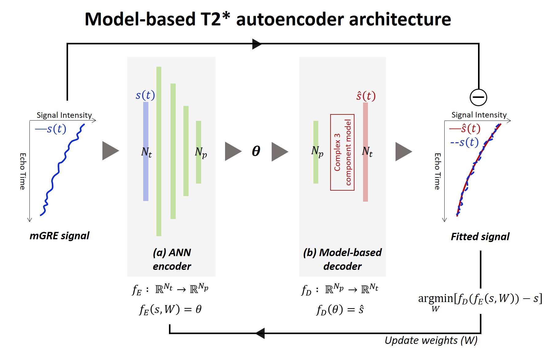

Figure 2. Histogram of model parameters (𝜽) for white matter region resulting from conventional curve-fitting (referred here as ‘conventional’) and model-based T2* autoencoder (referred here as ‘proposed’). (a) Amplitude, (b) T2* and (c) frequency offset of each water component. Note that the estimated T2* from conventional method are biased by the initial guess and/or upper bounds (red arrow).