1329
Time-resolved 3D Flow-MRF for relaxation and velocity quantification in the carotid arteries1Physikalisch-Technische Bundesanstalt Berlin (PTB), Braunschweig and Berlin, Germany, 2Medical Physics in Radiology, German Cancer Research Center (DKFZ), Heidelberg, Germany, 3Faculty of Physics and Astronomy, Heidelberg University, Heidelberg, Germany
Synopsis
The simultaneous quantification of blood velocity and tissue relaxation times could be a valuable tool for clinicians, especially in the carotid arteries, where atheroma plaques could occur. This can be achieved using the recently presented Flow-MRF technique that relies on the acquisition of randomly distributed gradients m1 momentum using a FISP MRF-sequence, with varying flip angle and fixed TR. In this work, Flow-MRF is extended to a time-resolved 3D acquisition and successfully applied in-vivo to the carotid bifurcation at 3T. T1, T2 and 3D time-resolved flow maps are recovered in a 3D slab.
Introduction
Atheroma plaque composition is a key factor to determine the risk for future cardiovascular events1,2. A simultaneous determination of blood flow in vessels and relaxation times of surrounding tissues could provide improved tissue characterization for advanced diagnostics. To that end, Magnetic Resonance Fingerprinting (MRF)3 has been adapted to enable time-resolved blood flow quantification within vessels for 2D acquisitions4. Furthermore, a 3D implementation of MRF with bipolar gradients was recently proposed5, however, the velocity assessment was limited to a time-averaged value over the brain. In this work, we extend the 2D Flow-MRF method to a stack-of-stars 3D acquisition, allowing the quantification of time-resolved 3D blood velocity vector fields, as well as T1 and T2 values of static tissues. We apply this technique to the carotid bifurcation at 3T.Materials and Methods
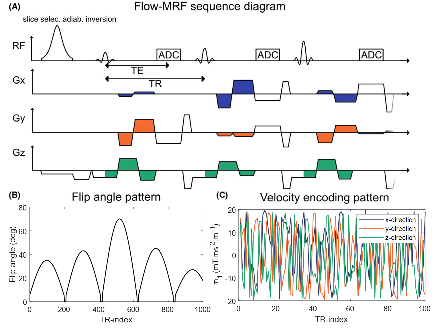
MRI acquisitionsA stack-of-stars6 FISP sequence was implemented with flow-encoding bipolar gradients in three directions, as illustrated in Fig.1. Here, pseudo-random first gradient moments (m1) with white-noise distributions between -20 and 20 mT/m.ms2 were applied (Fig.1c). Such acquisition strategy allows simultaneous velocity quantification in all directions, as well as T1 and T2 assessment based on the MRF method.
Scanning was performed at 3T (Magnetom Verio, Siemens Healthineers, Germany), using a 4-channel neck-coil. Data was acquired in transverse orientation with (300mm)2 in-plane field-of-view (FOV), (0.8mm)2 voxel size and 16mm slab thickness containing 8 slices. TR/TE were set to 8.95ms/5.95ms, with a bandwidth per pixel of 500Hz/px. Undersampled k-space data was retrieved using a radial multi-shot approach with a total number of 1000 time-frames acquired per shot. 10 shots rotated by golden angles (137.51°) were acquired per partition. An 8s delay was inserted between shots for thermal equilibrium recovery, leading to a total acquisition time of 23min18s. The top and bottom slice of the partition were not considered for further analysis due to slab aliasing.
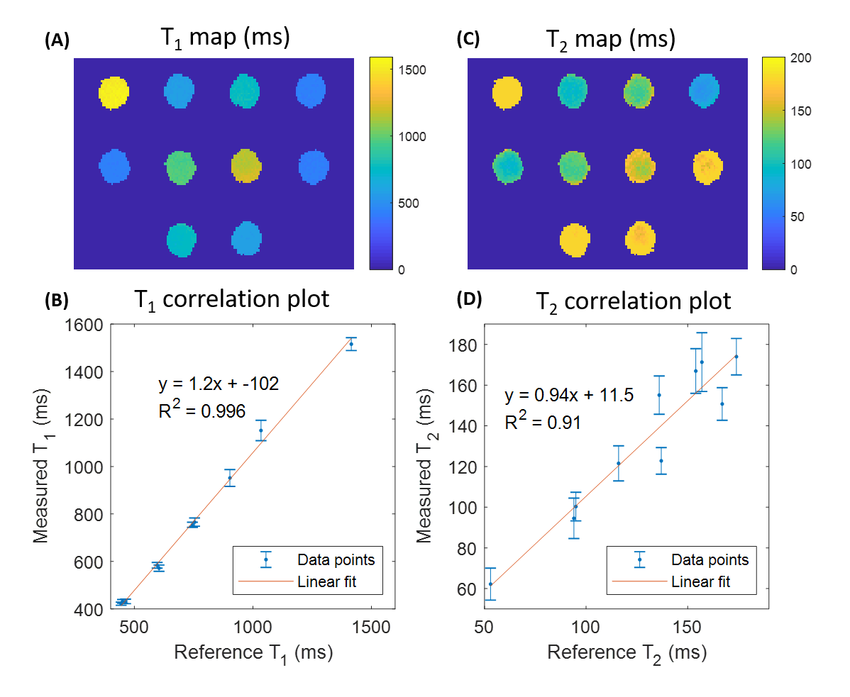
A relaxometric phantom (Diagnostics Sonar Ltd, Livingston, United Kingdom) consisting of 10 tubes with known nominal relaxation times was scanned to assess the reliability of T1 and T2 estimates.
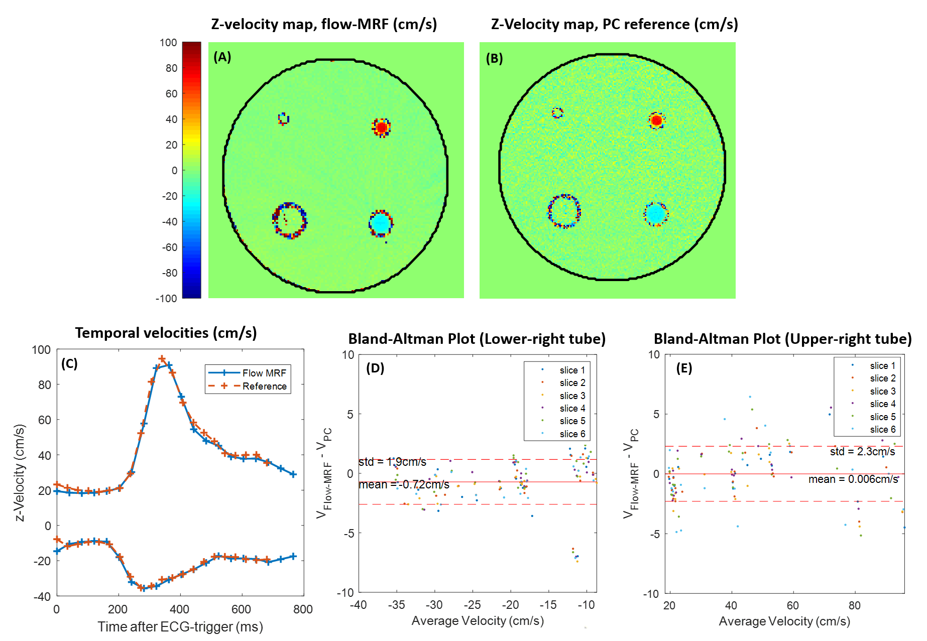
To assess velocity accuracy, two pipes of diameters 8 and 12mm immersed in a PVC phantom were connected to a pulsatile pump (CardioFlow 5000MR, Shelley, Canada) generating a carotid-like flow pattern. A reference flow acquisition was performed using a time-resolved 3D phase-contrast acquisition with three-directional velocity encoding (4Dflow) with a (160x160x16)mm3 FOV, (0.8x0.8x2)mm3 resolution, TR/TE=36.4/5.15ms, and a bandwidth of 300Hz/px. A GRAPPA factor of 2 was applied, leading to a total acquisition time of 12min45sec.
The presented 3D flow-MRF sequence was used to scan two healthy volunteers (male 28y.o., female 60y.o.), in accordance with local ethics regulations.
Quantitative extraction
The quantitative analysis was performed using MATLAB (Mathworks, Natick, USA). Voxel-wise estimates for T1 and T2 were determined using a low-rank alternating direction method of multipliers7 based approach. The range of simulated values for T1 and T2 were [300:5:3000]ms and [10:2:180]ms. The reconstruction included coil sensitivity maps calculated with the ESPIRiT method8, and B1 was assumed to be homogeneous in these 3T experiments.
To recover temporal 3D velocity fields, the acquisition was synchronized with ECG signal. Projections from the same cardiac phase were used jointly to assess time-resolved velocities as described by Flassbeck et al.4 with a temporal resolution of 40.2ms.
Results
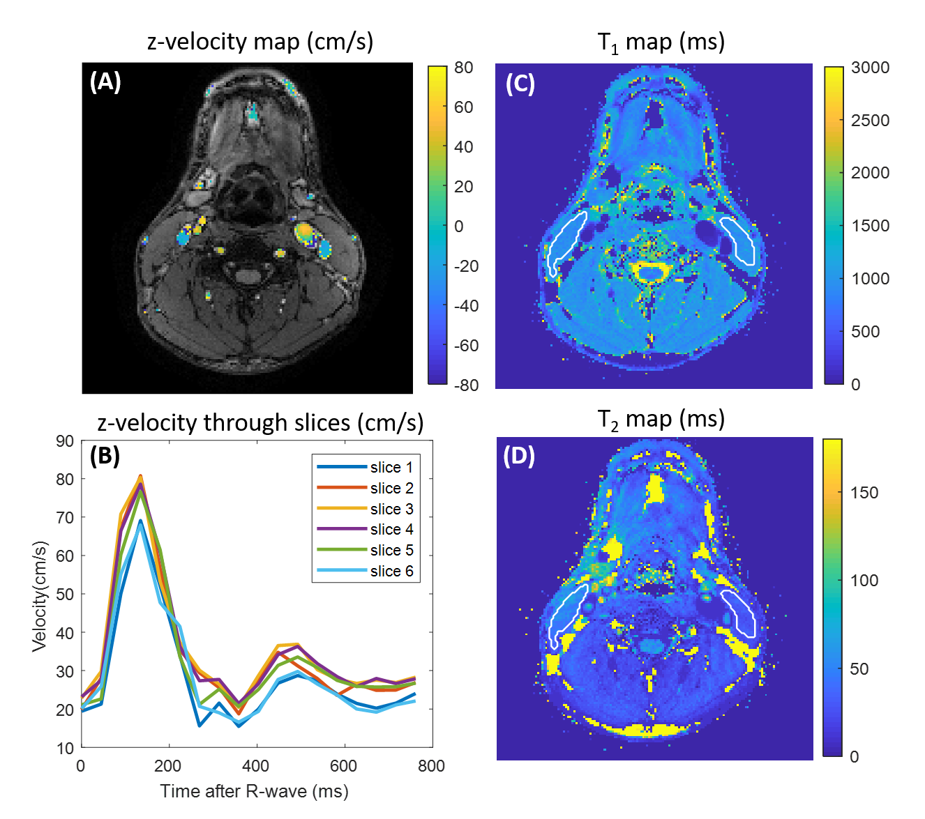
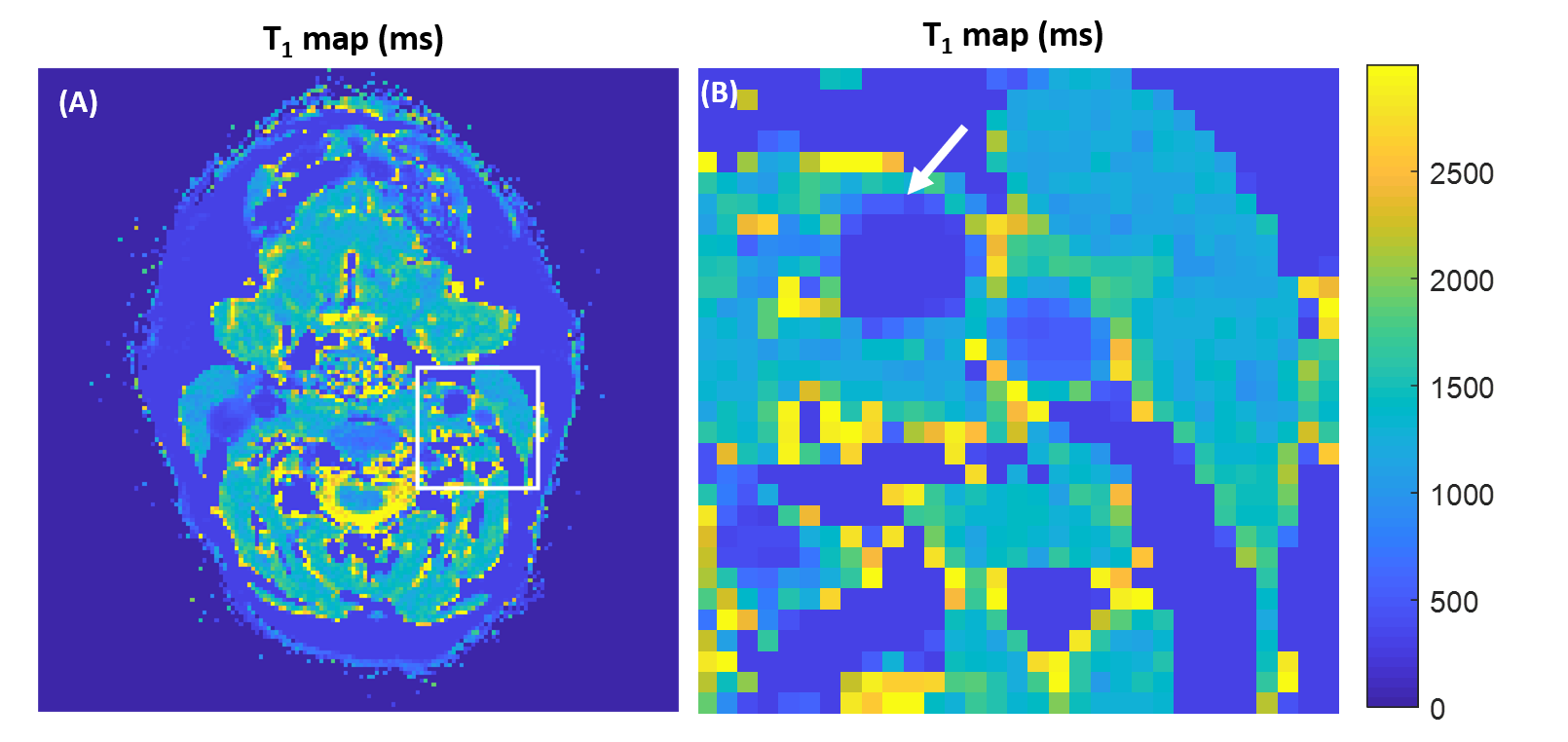
Relaxometric maps recovered in the multi-compartment phantom, displayed in Fig.2, demonstrate a good agreement with reference values provided by the manufacturer. Overall, a mean deviation of 2.0% and 5.9% for T1 and T2 assessments, respectively, were retrieved. Fig.3 displays the temporal velocity evolution assessed in both tested tubes. Bland-Altman analyses indicate a mean deviation of -0.72±1.9cm/s and -0.006±2.3cm/s between Flow-MRF and 4Dflow results in both tubes for the full range of tested velocities.In vivo temporal velocities assessed through the different slices are displayed in Fig.4. Measured peak velocity values correspond to the expected velocities in the carotid arteries9. Associated T1 and T2 in the surrounding sternocleidomastoid muscle are estimated to be 1169±68ms and 41±12ms, which agrees with previously reported values in the literature2 of T1=1137±110ms and T2=34±2ms. The resolution of the T1 maps are at the threshold where the carotid wall becomes visible despite a strong partial volume effect, as shown in Fig. 5 for the second subject.
Discussion
These results demonstrate the feasibility of 3D Flow-MRF to quantify 3D time-resolved velocity vector fields in the carotid bifurcation as well as 3D relaxometric maps of the surrounding static tissues.Extracted velocities and relaxometric values, both in-vitro and in-vivo, showed a good reliability over large targeted ranges. A larger standard deviation was observed for T2, which might be explained by the relatively long TE needed to incorporate flow-encoding gradients, leading to an increased sensitivity to Eddy currents and diffusion. Moreover, the inclusion of a B1+ map in the reconstruction, as has been done for 2D MRF at 7T4, is expected to enhance the results’ accuracy. Our preliminary result seem to reflect the carotid wall in the T1 maps despite a significant partial volume effect, however, higher resolution and matched anatomical images are required for clear delineation. Higher resolution and larger coverage are feasible using this framework and will be particularly beneficial for plaque characterization in combination with higher SNR provided by 7T.
Acknowledgements
No acknowledgement found.References
1. Hellings WE, Peeters W, Moll FL, Piers SRD, van Setten J, Van der Spek PJ, de Vries J-PPM, Seldenrijk KA, De Bruin PC, Vink A, et al. Composition of carotid atherosclerotic plaque is associated with cardiovascular outcome: a prognostic study. Circulation. 2010;121(17):1941–1950. doi:10.1161/CIRCULATIONAHA.109.887497
2. Coolen BF, Poot DHJ, Liem MI, Smits LP, Gao S, Kotek G, Klein S, Nederveen AJ. Three-dimensional quantitative T1 and T2 mapping of the carotid artery: Sequence design and in vivo feasibility. Magnetic Resonance in Medicine. 2016;75(3):1008–1017. doi:10.1002/mrm.25634
3. Ma D, Gulani V, Seiberlich N, Liu K, Sunshine JL, Duerk JL, Griswold MA. Magnetic resonance fingerprinting. Nature. 2013;495(7440):187–192. doi:10.1038/nature11971
4. Flassbeck S, Schmidt S, Bachert P, Ladd ME, Schmitter S. Flow MR fingerprinting. Magnetic Resonance in Medicine. 2018;81(4):2536–2550. doi:10.1002/mrm.27588
5. Portnoy S, Schrauben EM, Chau V, Macgowan CK. Flow-Encoded Magnetic Resonance Fingerprinting: Simultaneous Measurement of Flow, T1, & T2 with Whole Brain Coverage. In: Proc. Intl. Soc. Mag. Reson. Med. 27. 2018. p. 1103. http://cds.ismrm.org/ismrm-2008/files/01248.pdf
6. Peters DC, Korosec FR, Grist TM, Block WF, Holden JE, Vigen KK, Mistretta CA. Undersampled projection reconstruction applied to MR angiography. Magnetic Resonance in Medicine. 2000;43(1):91–101. doi:10.1002/(SICI)1522-2594(200001)43:1<91::AID-MRM11>3.0.CO;2-4
7. Assländer J, Cloos MA, Knoll F, Sodickson DK, Hennig J, Lattanzi R. Low rank alternating direction method of multipliers reconstruction for MR fingerprinting: Low Rank ADMM Reconstruction. Magnetic Resonance in Medicine. 2018;79(1):83–96. doi:10.1002/mrm.26639
8. Uecker M, Lai P, Murphy MJ, Virtue P, Elad M, Pauly JM, Vasanawala SS, Lustig M. ESPIRiT-an eigenvalue approach to autocalibrating parallel MRI: Where SENSE meets GRAPPA. Magnetic Resonance in Medicine. 2014;71(3):990–1001. doi:10.1002/mrm.24751
9. Harloff A, Albrecht F, Spreer J, et al. 3D blood flow characteristics in the carotid artery bifurcation assessed by flow-sensitive 4D MRI at 3T. Magnetic Resonance in Medicine 2009;61:65–74.
10. Jiang Y, Ma D, Seiberlich N, Gulani V, Griswold MA. MR fingerprinting using fast imaging with steady state precession (FISP) with spiral readout. Magnetic Resonance in Medicine. 2015;74(6):1621–1631. doi:10.1002/mrm.25559
Figures