Introduction

Myocardial perfusion MRI is an important tool to detect coronary artery disease. The clinical standard sequence requires a reliable ECG-gating signal, has limited slice coverage, and different cardiac phases in different slices. To address these limitations, we propose Continuous Radial Interleaved simultaneous Multi-slice acquisitions at sPoiled steady-state (CRIMP) that combines radial trajectory, simultaneous multi-slice (SMS), interleaving slice groups, and spoiled gradient echo (SPGR) readout. The sequence runs continuously without ECG-gating, breath-holding, or magnetization preparation (such as with a saturation recovery pulse). The sequence captures multiple cardiac phases in all of the image slices and keeps the magnetization of the inner slices in steady-state in spite of motion. The current work improves upon (1) by (i) using a novel reconstruction method, (ii) studying motion effects on the SPGR signal and (iii) performing perfusion quantification. We tested the sequence on 7 patients at both stress and rest, and performed a dual-bolus (2) scan at rest for quantitative analysis.

Methods

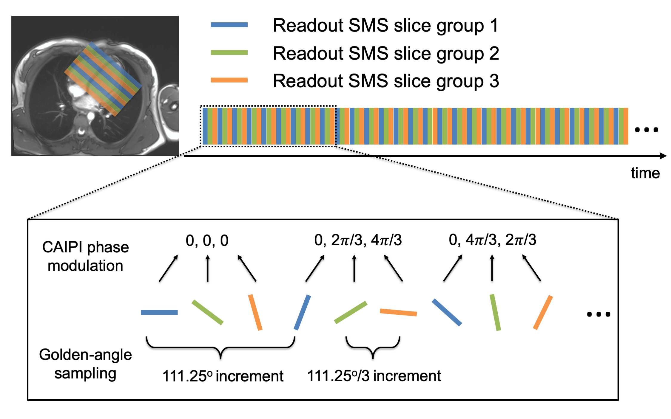
Pulse Sequence
The sequence interleaves three or four radial SMS slice groups ($$$N_{\mathrm{SG}}$$$) as shown in Figure 1. CAIPIRINHA (3) phase modulation is applied with a multi-slice factor $$$N_{\mathrm{SMS}}=3$$$, resulting in a total of 9 or 12 image slices. We apply a golden angle sampling (4) within each slice group, and use an offset angle of $$$111.25°/N_{\mathrm{SG}}$$$ between slice groups. All studies were performed on a 3T Prisma (Siemens) scanner with parameters: TR/TE=5.9/0.8ms, FOV=260mm², voxel size=1.8x1.8x5-8mm³ and FA=14°-15°.

Reconstruction
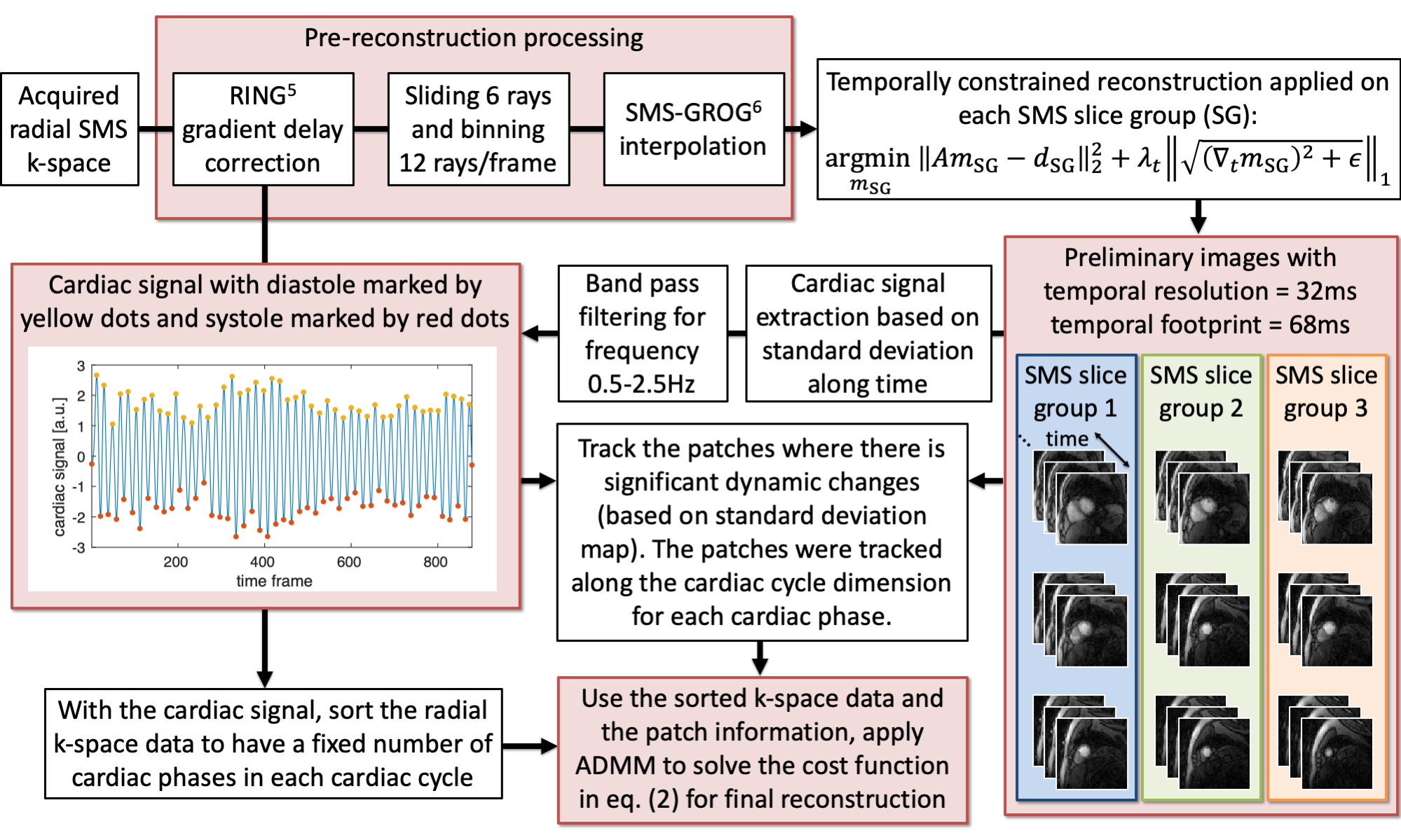
Image reconstruction was performed in two stages. In the first stage, we obtained preliminary images with a high temporal resolution for cardiac self-gating. We used the RING method (5) to correct for gradient delay errors. We then used a sliding-window that slides 6 rays and uses 12 rays/time frame to sort the data, achieving a temporal resolution of 32ms with a temporal footprint of 68ms. The sorted radial SMS k-space was interpolated onto a Cartesian grid by SMS-GROG (6). A temporally constrained reconstruction was used separately for each slice group (SG) by minimizing the cost function:
$$\underset{m_{\mathrm{SG}}}{\mathrm{argmin}}\left\Vert{A}m_{\mathrm{SG}}-d_{\mathrm{SG}}\right\Vert^2_2+\lambda_{t,\mathrm{SG}}\left\Vert\sqrt{(\nabla_tm_{\mathrm{SG}})^2}+\epsilon\right\Vert_1,(1)$$
where $$$A=\Phi DFS$$$ is the forward sampling matrix including sensitivity maps $$$S$$$, Fourier transform $$$F$$$, undersampling mask $$$D$$$, and phase modulation $$$\Phi$$$. $$$\lambda_{t,\mathrm{SG}}=0.04C$$$ with $$$C$$$ being the highest pixel intensity in the initial estimation $$$A^Hd_{\mathrm{SG}}$$$. The cardiac signal was automatically extracted from the preliminary images as shown in Figure 2. By using the cardiac signal, the radial k-space data was sorted to have a fixed number of cardiac phases in each cardiac cycle. Then motion-compensated patch-based total variation and locally low-rank regularizations were applied on each cardiac phase and included in the cost function in eq. (1) to finish the reconstruction, with all slices reconstructed jointly:
$$\underset{m}{\mathrm{argmin}}\left\Vert{A}m-d'\right\Vert^2_2+\lambda_t\left\Vert\sqrt{(\nabla_tm)^2}+\epsilon\right\Vert_1+\lambda_t\sum_{i=1}^{N_{\mathrm{patch}}}\left\Vert\sqrt{(\nabla_{t,\mathrm{cycle}}\mathcal{P}_i)^2+\epsilon}\right\Vert_1+\sum_{i=1}^{N_{\mathrm{patch}}}\left\Vert\mathcal{P}_i\right\Vert_*,s.t.\mathcal{P}_i=P_i(m).(2) $$
$$$\mathcal{P}_i=P_i(m)$$$ (of size $$$5\times5\times2\times{N}_{\mathrm{cycle}}$$$) represents the $$$i$$$th patch series extracted from the image $$$m$$$, and $$$\left\Vert\cdot\right\Vert_*$$$ is the nuclear norm. An ADMM algorithm (7) was used to solve the cost function in eq. (2).

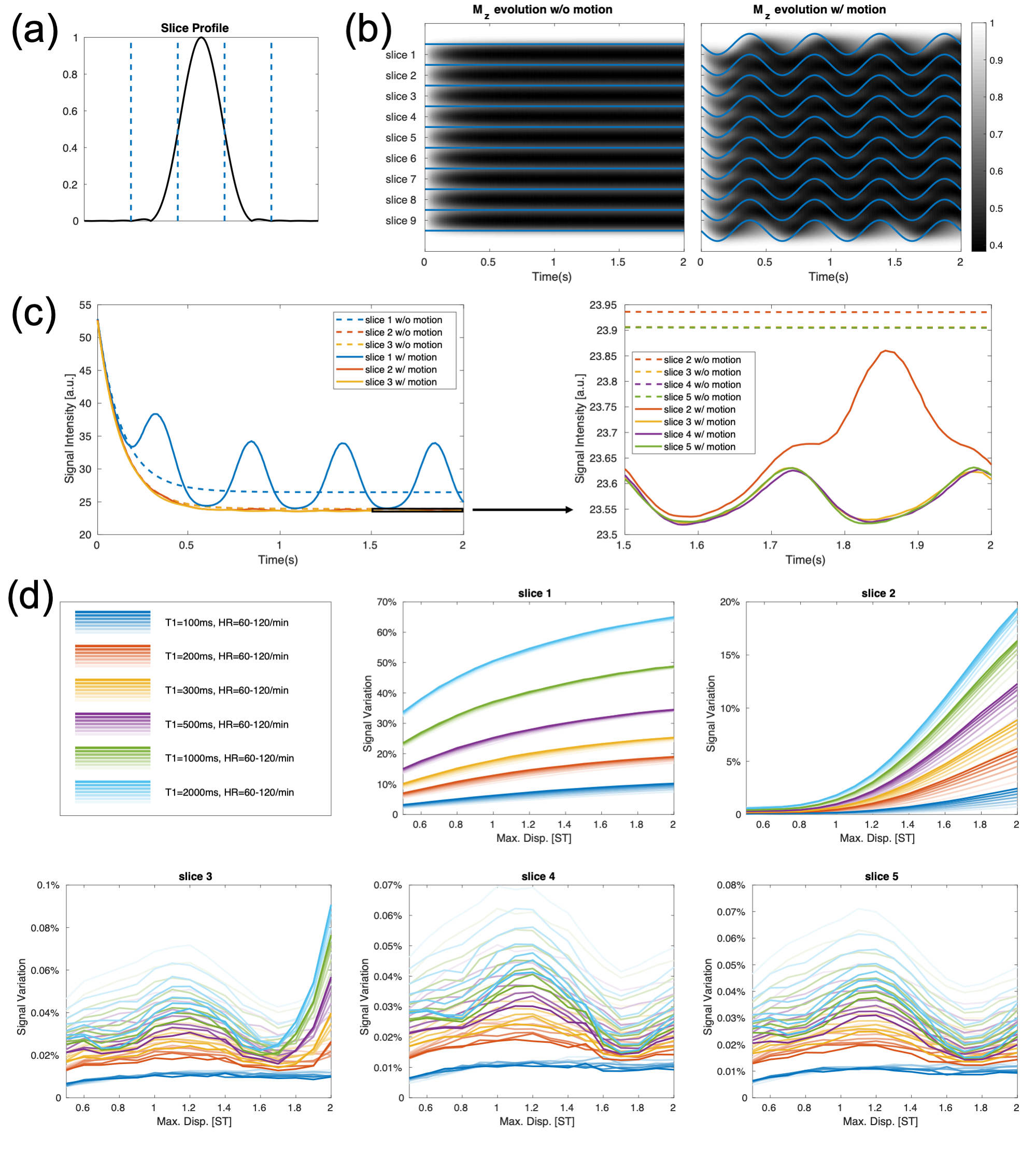
Simulation of Motion Effects on the Steady-State Signal
A potential issue with the SPGR readout is that the steady-state signal is sensitive to motion (8). We performed simulations to show that motion effects in CRIMP are ignorable for inner slices. A sinusoidal motion model with different heartrates and maximum displacements were used in the simulation.

Quantification
We obtained tissue curves from the CRIMP acquired images. The AIF was estimated from a separate diluted matched volume low-dose (0.0075mmol/L, 1/10 of the normal dose) injection acquired with a saturation recovery sequence proposed previously (6,9). Both the tissue and AIF signal intensity (SI) curves were converted to gadolinium concentration using a look-up-table created from Bloch simulations. CRIMP signal intensities were corrected for B1 inhomogeneity. We then fit the gadolinium curves to a two-compartment model to obtain the myocardial blood flow (MBF) values.

Results

Simulation of Motion Effects on the Steady-State Signal
The results summarized in Figure 3 show that the inner slices are less affected by motion than the outermost slices.

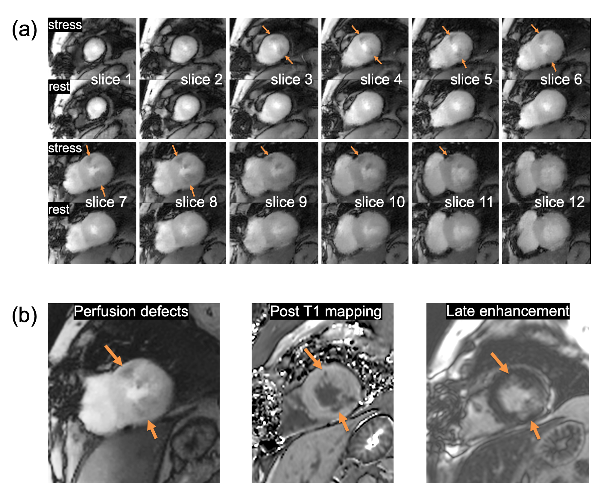
CRIMP acquired images with perfusion deficits
A total of 7 patients were scanned with CRIMP at both stress and rest. Figure 4 shows a subject with infarct acquired with 12 slices ($$$N_{\mathrm{SG}}=4$$$ and $$$N_{\mathrm{SMS}}=3$$$) and slice thickness=5mm. Figure 4(a) shows self-gated systolic images at myocardial enhancement for both stress and rest. Orange arrows point to perfusion deficits seen on the stress images. Figure 4(b) shows post-T1 and late enhancement images with a closely matched slice 7 with perfusion deficits.

Quantitative MBF
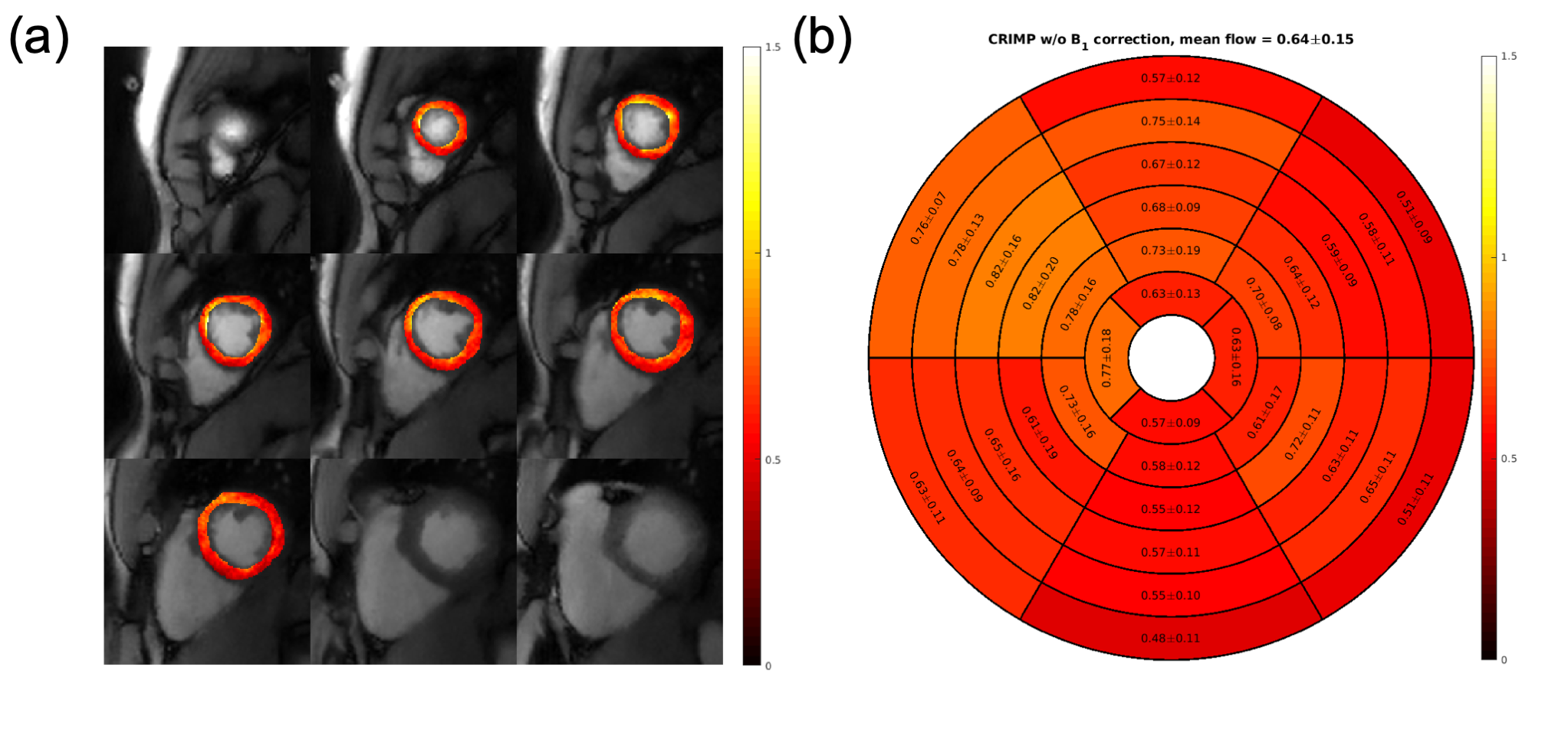
Figure 5 shows the systolic MBF maps estimated from the dual-bolus rest scan. Figure 5(a) shows pixelwise MBF and Figure 5(b) shows corresponding bullseye plots with segmentation according to the AHA 17-segment model (10). The averages MBF value is 0.64±0.15.

Discussion

CRIMP sequence can provide whole-heart coverage at multiple cardiac phases for first-pass myocardial perfusion without any ECG-gating or breath-holding, which has potential clinical benefits. However, the current reconstruction time requires ~3 hours, making the sequence less practical when timing is important. Another drawback of CRIMP is that the blood pool is affected by inflow effects, requiring a separate saturation recovery sequence to obtain the AIF. Given the whole-heart coverage with multiple cardiac phases and high SNR (1), the CRIMP sequence is advantageous for qualitative myocardial perfusion assessment.

Acknowledgements

This research was supported by the National Heart Lung and Blood Institute of the National Institutes of Health under award number RO1HL138082.