1306

Bayesian learning for fast parameter inference of multi-exponential white matter signals

Jonathan Doucette^1,2, Christian Kames^1,2, and Alexander Rauscher^1,3,4
¹UBC MRI Research Centre, Vancouver, BC, Canada, ²Department of Physics & Astronomy, University of British Columbia, Vancouver, BC, Canada, ³Department of Pediatrics, Faculty of Medicine, University of British Columbia, Vancouver, BC, Canada, ⁴Division of Neurology, Faculty of Medicine, University of British Columbia, Vancouver, BC, Canada

Synopsis

In this work we use Bayesian learning methods to investigate data-driven approaches to parameter inference of multi-exponential white matter signals. Multi spin-echo (MSE) signals are simulated by solving the Bloch-Torrey on 2D geometries containing myelinated axons, and a conditional variational autoencoder (CVAE) model is used to learn to map simulated signals to posterior parameter distributions. This approach allows for the mapping of MSE signals directly to physical parameter vectors without expensive post-processing. We demonstrate the effectiveness of this model through the simultaneous inference of the myelin water fraction, flip angle, intra-/extracullar water $$$T_2$$$, myelin water $$$T_2$$$, and myelin g-ratio.

Introduction

In vivo^1,2 assesment of the myelin water fraction (MWF) provides valuable insight into developmental myelination as well as degenerative demyelinating diseases^3–7. MWF measurements derived from multi spin-echo (MSE)-based myelin water imaging (MWI) correlate well with histology^8,9, however there remains no gold standard for in vivo MWF validation.

Traditional MSE MWI involves fitting signal relaxation models – which necessarily simplify the underlying physics – and inferring MWF based on model parameters. For example, modelling the MSE signal as a sum of exponentials permits the computation of a $$$T_2$$$-distribution using non-negative least squares curve-fitting (NNLS). This inverse problem is known to be difficult¹⁰, requiring appropriate regularization² and long computation times. Additionally, computing the MWF from the $$$T_2$$$-distribution requires choosing $$$T_2$$$ cutoff windows based on known ranges of intra/extra-cellular water (IEW) $$$T_2$$$ and myelin water (MW) $$$T_2$$$.

Here, we improve on previous MSE-based methods by combining MSE signal simulation with data-driven learning of signal dynamics. MSE signals are simulated by solving the Bloch-Torrey (BT) equation¹¹ on 2D geometries containing myelinated axons, removing simplifying model assumptions on the signal shape. Data-driven learning on simulated signals allows for the mapping of MSE signals directly to physical parameters such as MWF – without expensive calculations such as NNLS – leading to fast whole-brain parameter inference. By training on simulated signals, we also remove the issue of choosing a gold standard method to compare with, as e.g. the MWF is known from the simulation geometry.

Methods

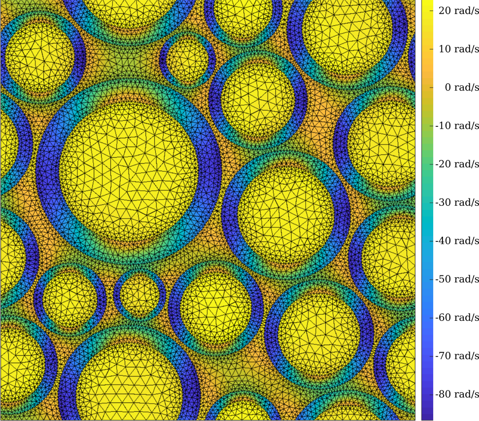
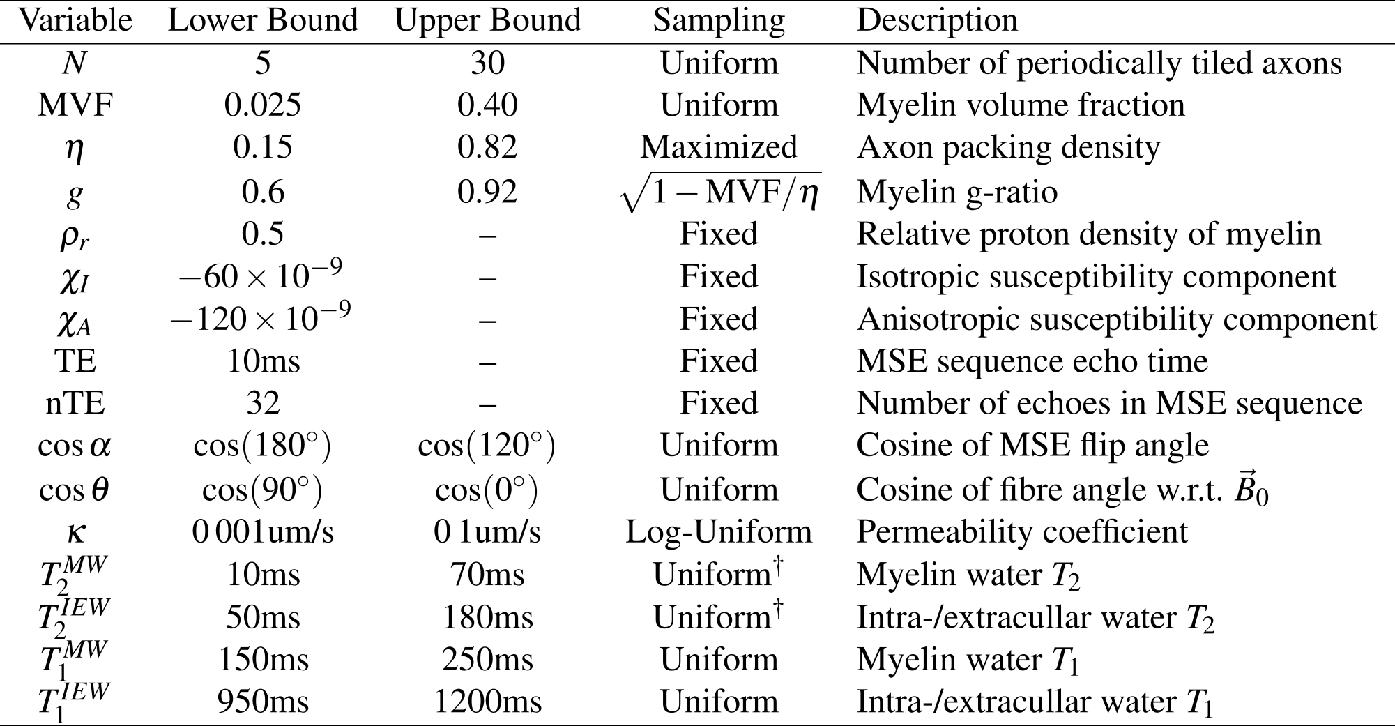
Two-dimensional grids containing myelinated axons tiled periodically were generated programmatically, as in Figure 1. Each grid was simulated from 4 parameters: number of axons $$$N$$$, myelin volume fraction (MVF), packing density $$$\eta$$$, and g-ratio $$$g$$$. $$$N$$$ and MVF were chosen uniformly from their ranges in Table 1. For a given MVF, $$$\eta$$$ is chosen maximally among feasible values. $$$g$$$ is determined by $$$\text{MVF}=(1-g^2)\,\eta$$$. Note: the relative proton density of myelin $$$\rho_r=0.5$$$ implies $$$\text{MWF}=\text{MVF}/(2-\text{MVF})$$$.

Simulated MSE signals are generated through solving the BT equation, the strong form of which is given by $$\begin{cases}\frac{\partial{}}{\partial{}t}M_x=\nabla{}\cdot{}(D\nabla{}M_x)-R_2\,M_x+\omega\,M_y\\\frac{\partial{}}{\partial{}t}M_y=\nabla{}\cdot{}(D\nabla{}M_y)-R_2\,M_y-\omega\,M_x\\\frac{\partial{}}{\partial{}t}M_z=\nabla{}\cdot{}(D\nabla{}M_z)-R_1\,(M_z-M_{z,\infty})\end{cases}$$ where the diffusivity $$$D(x)$$$, relaxation rates $$$R_1(x)$$$ and $$$R_2(x)$$$, and resonance frequency $$$\omega(x)$$$ are functions of position, and $$$\vec{M}(x,t)=[M_x(x,t),\,M_y(x,t),\,M_z(x,t)]$$$ is the magnetization vector. $$$\omega(x)$$$ is given by the sum over individual fibre fields, each computed in closed form using the hollow cylinder model¹². Letting $$$\vec{u}(x,t)=[M_x(x,t),\,M_y(x,t),\,M_{z,\infty}-M_z(x,t)]$$$, the corresponding weak formulation is $$\frac{\partial}{\partial{}t}\int_{\Omega}\vec{v}\cdot\vec{u}\,d\Omega=-\int_{\Omega}\nabla\vec{v}:D\,\nabla\vec{u}+\vec{v}\cdot(\vec{R}\odot\vec{u})-\omega\,\vec{v}_\perp\times\vec{u}_\perp\,d\Omega$$ where $$$\Omega$$$ is the domain, $$$\vec{v}$$$ is a test function, $$$:$$$ denotes tensor contraction, $$$\odot$$$ denotes elementwise multiplication, $$$\perp$$$ denotes the transverse component, $$$\times$$$ denotes the scalar two-dimensional cross product, and $$$\vec{R}(x)=[R_2(x),\,R_2(x),\,R_1(x)]$$$. Reflecting boundary conditions are prescribed at the domain boundary; semi-permeable boundaries are implemented on the inner and outer walls of the myelin sheaths via 1D interface elements and a permeability coefficient $$$\kappa$$$¹³; linear basis functions and triangular elements were used to discretize the problem; mass and stiffness matrices were built using the Julia¹⁴ package JuAFEM.jl; the discretized system of ordinary differential equations was solved using the Expokit algorithm¹⁵ via the Julia packages Expokit.jl and DifferentialEquations.jl¹⁶.

Data-driven learning is performed using instances of the above simulations as training data, with parameters drawn from the distributions in Table 1. We use the convolutional variational autoencoder (CVAE) model detailed previously¹⁷ to learn the mapping from MSE signal space to sampleable posterior distributions over parameter space. These sampleable distributions are then used to compute voxelwise parameter statistics. The CVAE consists of three subcomponents: two encoders $$$E_1$$$, $$$E_2$$$ and a decoder $$$D$$$. Each component is implemented as 6 fully connected layers with 128 neurons per layer. $$$E_1$$$ learns to map input signal vectors $$$y$$$ to intermediate distributions over a latent variable space $$$Z$$$; $$$E_2$$$ also maps $$$y$$$ to distributions on $$$Z$$$, but is additionally informed by the goal parameters $$$x$$$; $$$D$$$ learns the mapping from $$$Z$$$ to parameter space. During training the cross-entropy $$H\lesssim-\frac{1}{N_B}\sum_{i=1}^{N_B}\log{}D(x_i|z_i,y_i)-\text{KL}[E_2(z|x_i,y_i)\,||\,E_1(z|y_i)]$$ is minimized over minibatches of size $$$N_B=250$$$, where $$$\text{KL}(\cdot||\cdot)$$$ is the Kullback-Leibler divergence¹⁸. During testing, samples $$$x$$$ are repeatedly drawn via $$$y\rightarrow{}E_1\rightarrow{}Z\rightarrow{}D\rightarrow{}x$$$. Using this model, we learn to map MSE signals to distributions over 5 parameters: cosine of the MSE flip angle $$$\cos\alpha$$$, $$$g$$$, MWF, $$$T_2^{MW}/\text{TE}$$$, and $$$T_2^{IEW}/\text{TE}$$$, where TE is the echotime.

Discussion and conclusion

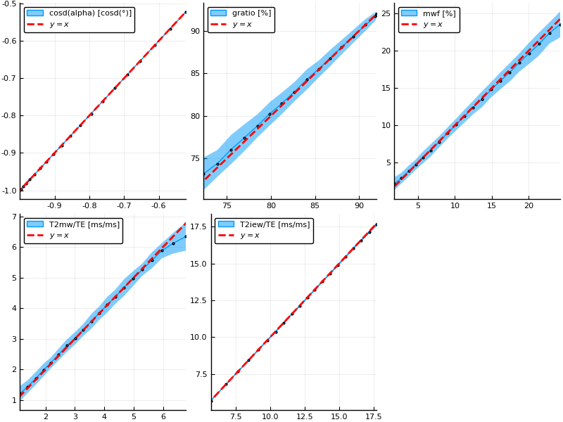
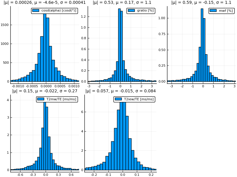
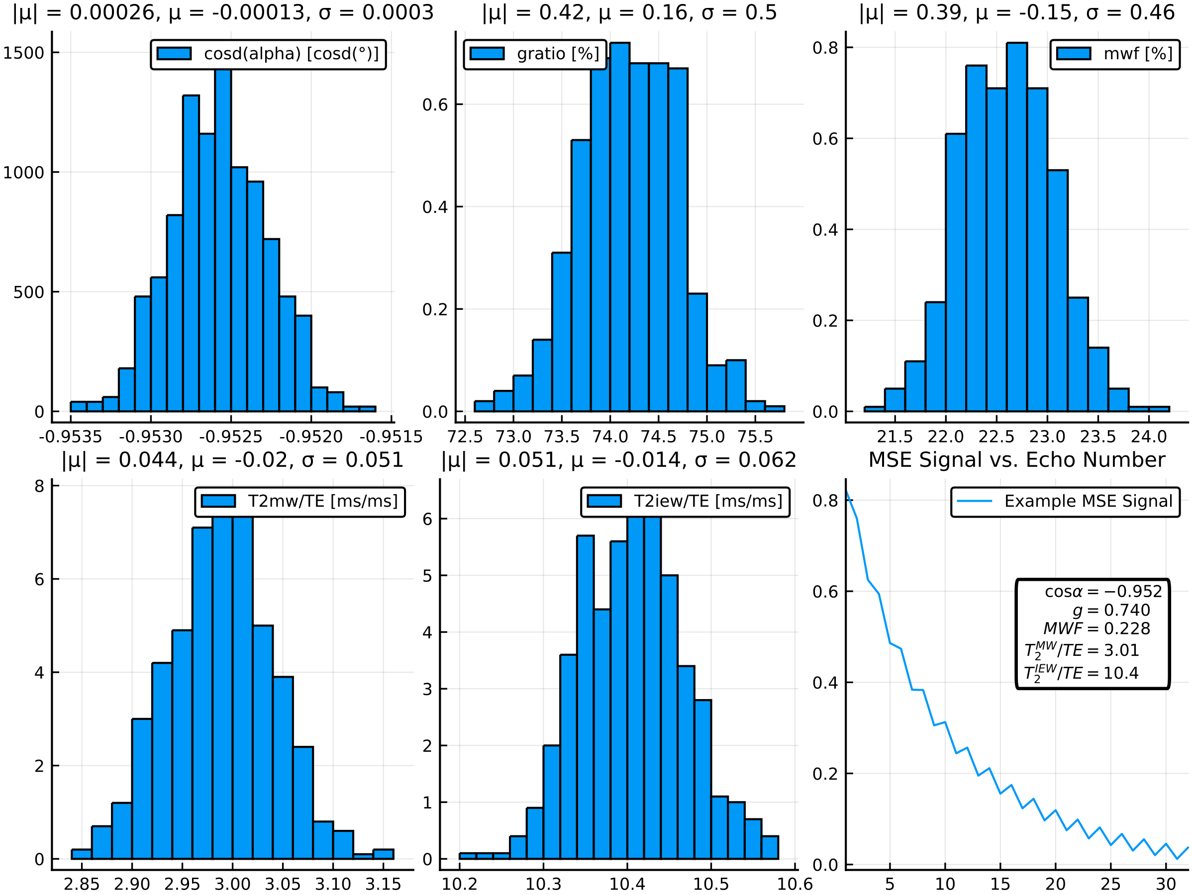
Figure 2 shows parameter inference results on the test data set. Inference recovers $$$\cos\alpha$$$ and $$$T_2^{IEW}$$$ with high accuracy; intuitively, this is due to their having the largest effect on the signal shape. $$$T_2^{MW}$$$, $$$g$$$, and MWF are inferred with mutually similar but lower accuracies, as they have smaller effects on the signal shape. Figure 3 quantifies the inference errors: $$$\cos\alpha$$$, $$$g$$$, MWF, $$$T_2^{MW}/TE$$$, and $$$T_2^{MW}/TE$$$ are inferred with 1-$$$\sigma$$$ inference errors of 0.00041, 1.1%, 1.1%, 0.27 ms/ms, and 0.084 ms/ms, respectively. Figure 4 shows an example simulated MSE signal and corresponding parameter posterior distributions from the CVAE model, illustrating the ability to compute arbitrary voxelwise statistics.

The proposed Bayesian learning approach allows one to embed any number of inferable parameters into the latent variable space during training, resulting in flexible and fast parameter inference which requires neither expensive fitting procedures nor simplified models of the underlying signal.

Acknowledgements

Natural Sciences and Engineering Research Council of Canada, Grant/Award Number 016-05371, and the Canadian Institutes of Health Research, Grant Number RN382474-418628.

References

[1] A. Mackay, K. Whittall, J. Adler, D. Li, D. Paty, and D. Graeb, “In vivo visualization of myelin water in brain by magnetic resonance,” Magnetic Resonance in Medicine, vol. 31, no. 6, pp. 673–677, 1994.

[2] K. P. Whittall, A. L. Mackay, D. A. Graeb, R. A. Nugent, D. K. B. Li, and D. W. Paty, “In vivo measurement of T2 distributions and water contents in normal human brain,” Magnetic Resonance in Medicine, vol. 37, no. 1, pp. 34–43, 1997.

[3] I. R. Levesque and G. B. Pike, “Characterizing healthy and diseased white matter using quantitative magnetization transfer and multicomponent T2 relaxometry: A unified view via a four-pool model,” Magnetic Resonance in Medicine, vol. 62, no. 6, pp. 1487–1496, 2009.

[4] A. L. MacKay and C. Laule, “Magnetic Resonance of Myelin Water: An in vivo Marker for Myelin,” Brain Plasticity, vol. 2, no. 1, pp. 71–91, Jan. 2016.

[5] A. MacKay, C. Laule, I. Vavasour, T. Bjarnason, S. Kolind, and B. Mädler, “Insights into brain microstructure from the T2 distribution,” Magnetic Resonance Imaging, vol. 24, no. 4, pp. 515–525, May 2006.

[6] E. Alonso-Ortiz, I. R. Levesque, and G. B. Pike, “MRI-based myelin water imaging: A technical review,” Magnetic Resonance in Medicine, vol. 73, no. 1, pp. 70–81, 2015.

[7] C. Birkl, A. M. Birkl-Toeglhofer, V. Endmayr, R. Höftberger, G. Kasprian, C. Krebs, J. Haybaeck, and A. Rauscher, “The influence of brain iron on myelin water imaging,” NeuroImage, vol. 199, pp. 545–552, 2019.

[8] P. Kozlowski, D. Raj, J. Liu, C. Lam, A. C. Yung, and W. Tetzlaff, “Characterizing White Matter Damage in Rat Spinal Cord with Quantitative MRI and Histology,” Journal of Neurotrauma, vol. 25, no. 6, pp. 653–676, Jun. 2008.

[9] C. Laule, E. Leung, D. K. Li, A. L. Traboulsee, D. W. Paty, A. L. MacKay, and G. R. Moore, “Myelin water imaging in multiple sclerosis: quantitative correlations with histopathology,” Multiple Sclerosis Journal, vol. 12, no. 6, pp. 747–753, Nov. 2006.

[10] A. A. Istratov and O. F. Vyvenko, “Exponential analysis in physical phenomena,” Review of Scientific Instruments, vol. 70, no. 2, pp. 1233–1257, Feb. 1999.

[11] H. C. Torrey, “Bloch Equations with Diffusion Terms,” Physical Review, vol. 104, no. 3, pp. 563–565, Nov. 1956.

[12] S. Wharton and R. Bowtell, “Fiber orientation-dependent white matter contrast in gradient echo MRI,” Proceedings of the National Academy of Sciences of the United States of America, vol. 109, no. 45, pp. 18559–18564, Nov. 2012.

[13] D. V. Nguyen, J.-R. Li, D. Grebenkov, and D. Le Bihan, “A Finite Elements Method to Solve the Bloch-Torrey Equation Applied to Diffusion Magnetic Resonance Imaging,” J. Comput. Phys., vol. 263, pp. 283–302, Apr. 2014.

[14] J. Bezanson, A. Edelman, S. Karpinski, and V. Shah, “Julia: A Fresh Approach to Numerical Computing,” SIAM Review, vol. 59, no. 1, pp. 65–98, Jan. 2017.

[15] R. B. Sidje, “Expokit: A Software Package for Computing Matrix Exponentials,” ACM Trans. Math. Softw., vol. 24, no. 1, pp. 130–156, Mar. 1998.

[16] C. Rackauckas and Q. Nie, “DifferentialEquations.jl – A Performant and Feature-Rich Ecosystem for Solving Differential Equations in Julia,” Journal of Open Research Software, vol. 5, no. 1, p. 15, May 2017.

[17] H. Gabbard, C. Messenger, I. S. Heng, F. Tonolini, and R. Murray-Smith, “Bayesian parameter estimation using conditional variational autoencoders for gravitational-wave astronomy,” arXiv:1909.06296 [astro-ph, physics:gr-qc], Sep. 2019.

[18] S. Kullback and R. A. Leibler, “On Information and Sufficiency,” The Annals of Mathematical Statistics, vol. 22, no. 1, pp. 79–86, Mar. 1951.

Figures

Figure 1: Example simulated geometry with $$$N=15$$$ periodically tiled fibres, packing density $$$\eta=0.78$$$, g-ratio $$$g=0.78$$$ of the myelin sheath, myelin volume fraction $$$\text{MVF}=0.31$$$, and myelin water fraction $$$\text{MWF}=0.18$$$. Grid elements are coloured by $$$\omega(x)$$$, computed using the hollow cylinder model¹² for fibres perpendicular to a $$$B_0=3T$$$ magnetic field.

Figure 2: Inferred parameter values vs. true values over the test data set. Parameter values were sorted and partitioned into 20 equally sized subsets for visualization. Solid points represent mean values over subsets; ribbons represent 1-$$$\sigma$$$ ranges over subsets. $$$\cos\alpha$$$ and $$$T_2^{IEW}/TE$$$ are nearly exactly recovered. $$$g$$$, MWF, and $$$T_2^{MW}/TE$$$ are recovered with a mutually similar but lower accuracy. Note that for large $$$T_2^{MW}/TE$$$ the signal becomes more monoexponential, and therefore $$$T_2^{MW}/TE$$$ is harder to recover.

Figure 3: Normalized histograms of inferred parameter errors over the test data set. For each plot, $$$|\mu|$$$ is the mean absolute error, $$$\mu$$$ is the mean error or bias, and $$$\sigma$$$ is the standard deviation of the error.

Figure 4: Normalized histograms of inferred parameter posteriors for a single example MSE signal. For each plot, $$$|\mu|$$$ is the mean absolute error, $$$\mu$$$ is the mean error or bias, and $$$\sigma$$$ is the standard deviation of the error. On the bottom right is an example MSE signal which was input into the CVAE model. 1000 parameter inferences were then drawn from the respective posteriors, shown by the 5 histograms. Note that the true values, as seen in the bottom right figure, lie in the center of the respective distributions.

Table 1: Physical parameter values used during simulations. Lower- and upper bounds refer to sampling ranges. Fixed parameters are shown with no upper bound. $$${}^\dagger$$$During sampling, $$$T_2^{IEW}$$$ is constrained to be at least 1.5X larger than $$$T_2^{MW}$$$ in order to prevent degeneration into a monoexponential signal.

Proc. Intl. Soc. Mag. Reson. Med. 28 (2020)

1306