1298
Quantification of Non-Water-Suppressed Proton Spectroscopy using Deep Neural Networks
Marcia Sahaya Louis1, Eduardo Coello2, Huijun Liao2, Ajay Joshi3, and Alexander Lin2
1ECE, Boston University, Boston, MA, United States, 2Radiology, Brigham and Women's hospital, Boston, MA, United States, 3Boston University, Boston, MA, United States
1ECE, Boston University, Boston, MA, United States, 2Radiology, Brigham and Women's hospital, Boston, MA, United States, 3Boston University, Boston, MA, United States
Synopsis
Water is present in the brain tissue at a concentration that is at least four orders of magnitude higher than metabolites of interest. As a result, it is necessary to suppress the water resonance so that the brain metabolites of interest can be better visualized and quantified. This work presents a neural network model for extracting the metabolites spectrum from non-water-suppressed proton magnetic resonance spectra. The autoencoder model learns a vector field for mapping the water signal to a lower-dimensional manifold and accurately reconstructs the metabolite spectra as compared to water-suppressed spectra from the same subject.
Introduction
Magnetic Resonance Spectroscopy (MRS) is a specialized MR method that can non-invasively quantify metabolites in body tissues. However, the metabolites of interest acquired using MRS have a low concentration in the brain (∼1-15 mM), which is four orders of magnitude lower than the water concentration in tissue (∼35-50 M)1. Specialized sequences can suppress the high water signal2,3; however, the effectiveness of the water suppression is variable from patient to patient and can also result in the inadvertent suppression of resonances close to the water peak and/or lineshape distortion due to incompletely suppressed water signal. These issues cause biases in the current models and tools used to quantify the MRS data4–6. Therefore, it would be ideal to acquire MRS data without water suppression and utilize post-acquisition methods to eliminate the water signal. Methods such as Hankel singular value decomposition (HSVD)7 have been applied with mixed results. Modern deep learning models provide a framework to learn complex functions by mapping an input vector to an output vector, given sufficiently large datasets of labeled training examples8. This work presents an autoencoder model to remove water resonance from a water signal and extract the metabolite spectrum. The autoencoder predicted spectrum is quantified using LCModel5.Methods
The architecture of the autoencoder model is shown in Figure 1. The architecture has two sub-networks: encoder and decoder with a latent vector. The encoder network extracts spectral features from the water signal and compresses it to a lower-dimensional manifold (z), and the decoder network reconstructs the metabolite spectrum using the z. With this approach, the model learns a vector field for mapping the input water signal to z and is trained to effectively “cancel out” the water resonance.We created a synthetic dataset using a basis set of N-acetyl-aspartate (NAA), choline (Cho), creatine (Cr), glutamate(Glu), glutamine (Gln), myo-inositol (mI), glutathione (GSH) and gamma amino butyric acid (GABA). A synthetic FID is generated by performing a linear combination of the eight metabolites using random concentration values within human variance as weights9. The synthetic FID is Fourier transformed to obtain the metabolite spectra used as the reconstruction target spectra for the autoencoder model. The metabolite spectra are added to water spectra from in-vivo acquisitions to generate the input spectra for the autoencoder model. The synthetic data generation setup was used to generate synthetic datasets with varying water concentrations and synthetic noise from a random Gaussian distribution. Each dataset has a total of 10000 simulated input and target spectra and randomly divided 80% training set,10% validation set, and 10% test set. The autoencoder model was trained using Tensorflow10 with Keras as high-level API with the Adam optimizer and the maximum number of epochs set to 5000.
We used in-vivo data acquired in 487 scans to evaluate the autoencoder model. The data were acquired at 3T MRI using point-resolved (PRESS) single voxel spectroscopy (TE=30ms, TR=2s, 128 averages, 8 cc volume). The spectra were frequency corrected and spectral width aligned using OpenMRSLab11. The in-vivo dataset was randomly divided into a 67% training set and a 33% test set. The autoencoder model trained using a synthetic dataset was re-trained with the in-vivo dataset to improve the quality of the predicted spectrum. We increased the number of data samples in the training set by using a data augmentation technique where a new sample was generated by adding two different spectra to further improve the prediction of the autoencoder model. The autoencoder reconstructed spectrum, and the test set was then quantified using LCModel.
Results
We evaluated the reconstruction accuracy of the autoencoder model using the synthetic spectrum. Figure 2 shows the results of the noise analysis, the quality of the reconstructed spectrum is acceptable and similar to the target spectrum even for the input spectrum with considerable noise. The water removal capacity of the autoencoder model was evaluated by comparing it to the HSVD method, as shown in Figure 3. The reconstruction error is MAE=0.013 for the autoencoder model on the synthetic dataset. Figure 4 shows the results of the correlation between the autoencoder reconstructed and water suppressed spectrum for the in-vivo dataset. A correlation coefficient of R=0.9 was achieved between the water suppressed and the reconstructed spectrum in the in-vivo test set. Figure 5 shows the LCModel fitting for the spectrum with a correlation of R=0.99 and R=0.7.Conclusion
This work presented a machine learning approach for water removal. The autoencoder model was capable of fully removing the water signal to reconstruct the underlying metabolite spectrum. This allows for acquiring spectra without water suppression. Spectra acquired without water suppression has the advantage of providing an internal reference for quantification. It is particularly advantageous in MRSI12 methods by eliminating a second time-consuming reference scan.Acknowledgements
This work was supported by grants from the Partners Innovation Discovery Grants 2019.References
- Govindaraju, V., Young, K. & Maudsley, A. A. Proton NMR chemical shifts and coupling constants for brain metabolites. NMR in Biomedicine: An International Journal Devoted to the Development and Application of Magnetic Resonance In Vivo 13, 129–153 (2000)
- Tka´c, I., Star ˇ cuk, Z., Choi, I.-Y. & Gruetter, R. In vivo 1h NMR spectroscopy of rat brain at 1 ms echo time. ˇ Magnetic Resonance in Medicine: An Official Journal of the International Society for Magnetic Resonance in Medicine 41, 649–656 (1999).
- Ogg, R. J., Kingsley, R. & Taylor, J. S. Wet, a t1-and b1-insensitive water-suppression method for in vivo localized 1h NMR spectroscopy. Journal of Magnetic Resonance, Series B 104, 1–10 (1994).
- Wilson, M., Reynolds, G., Kauppinen, R. A., Arvanitis, T. N. & Peet, A. C. A constrained least-squares approach to the automated quantitation of in vivo 1h magnetic resonance spectroscopy data. Magnetic resonance in medicine 65, 1–12 (2011).
- Provencher, S. W. Automatic quantitation of localized in vivo 1h spectra with LCModel. NMR in Biomedicine 14, 260–264 (2001)
- Soher, B., Semanchuk, P., Todd, D., Steinberg, J. & Young, K. Vespa: integrated applications for rf pulse design, spectral simulation and MRS data analysis. In Proc Int Soc Magn Reson Med, vol. 19, 1410 (2011).
- Cabanes, E., Confort-Gouny, S., Le Fur, Y., Simond, G. & Cozzone, P. Optimization of residual water signal removal by HLSVD on simulated short echo time proton MR spectra of the human brain. Journal of Magnetic Resonance 150, 116–125 (2001).
- Goodfellow, I., Bengio, Y. & Courville, A. Deep learning (MIT press, 2016).
- De Graaf, R. A. In vivo NMR spectroscopy: principles and techniques (John Wiley & Sons, 2019).
- Abadi, M. et al. Tensorflow: A system for large-scale machine learning. In 12th {USENIX} Symposium on Operating Systems Design and Implementation ({OSDI} 16), 265–283 (2016).
- Rowland B, I. J. L. A., Mariano LJ. An open-source software repository for magnetic resonance spectroscopy data analysis tools. International Society for Magnetic Resonance in Medicine MR Spectroscopy Workshop (2016).
- Gasparovic, C. et al. Use of tissue water as a concentration reference for proton spectroscopic imaging. Magnetic Resonance in Medicine: An Official Journal of the International Society for Magnetic Resonance in Medicine 55, 1219–1226 (2006).
Figures
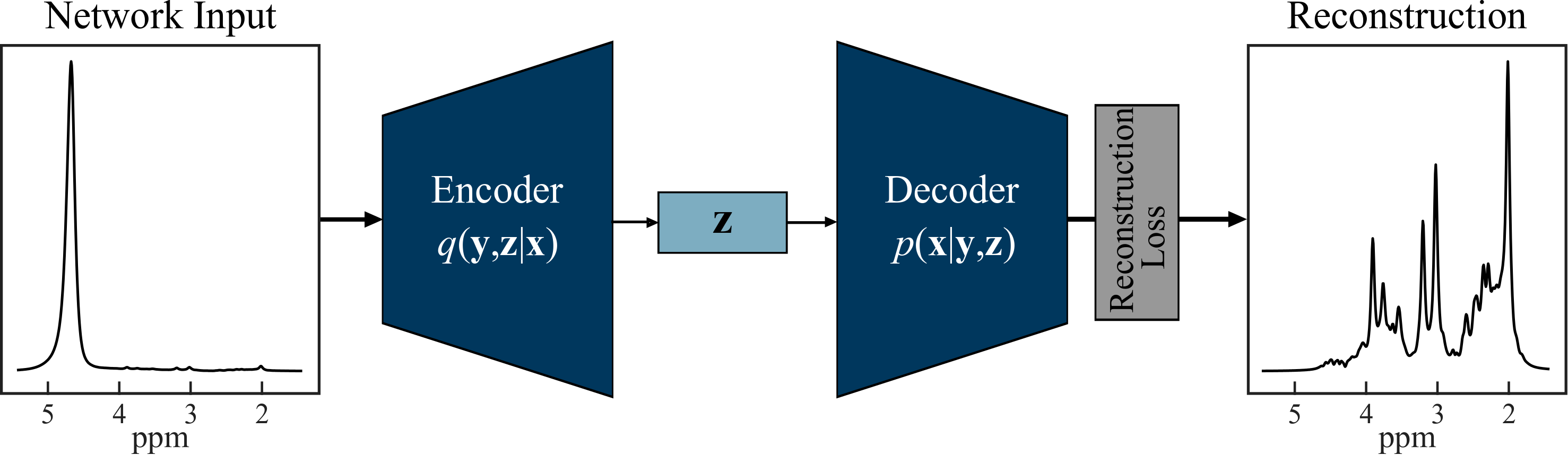
Autoencoder model for water removal. The encoder q(y,z|x) and decoder p(x|y,z) each have two 1D-convolutional layers with a kernel size of 3 and 16 filters and one fully connected layer with 1000 hidden units. All the layers in the model have a ReLU activation function, except the last layer has a tanh activation function. The latent vector (z) has 32 hidden units with a linear activation function.
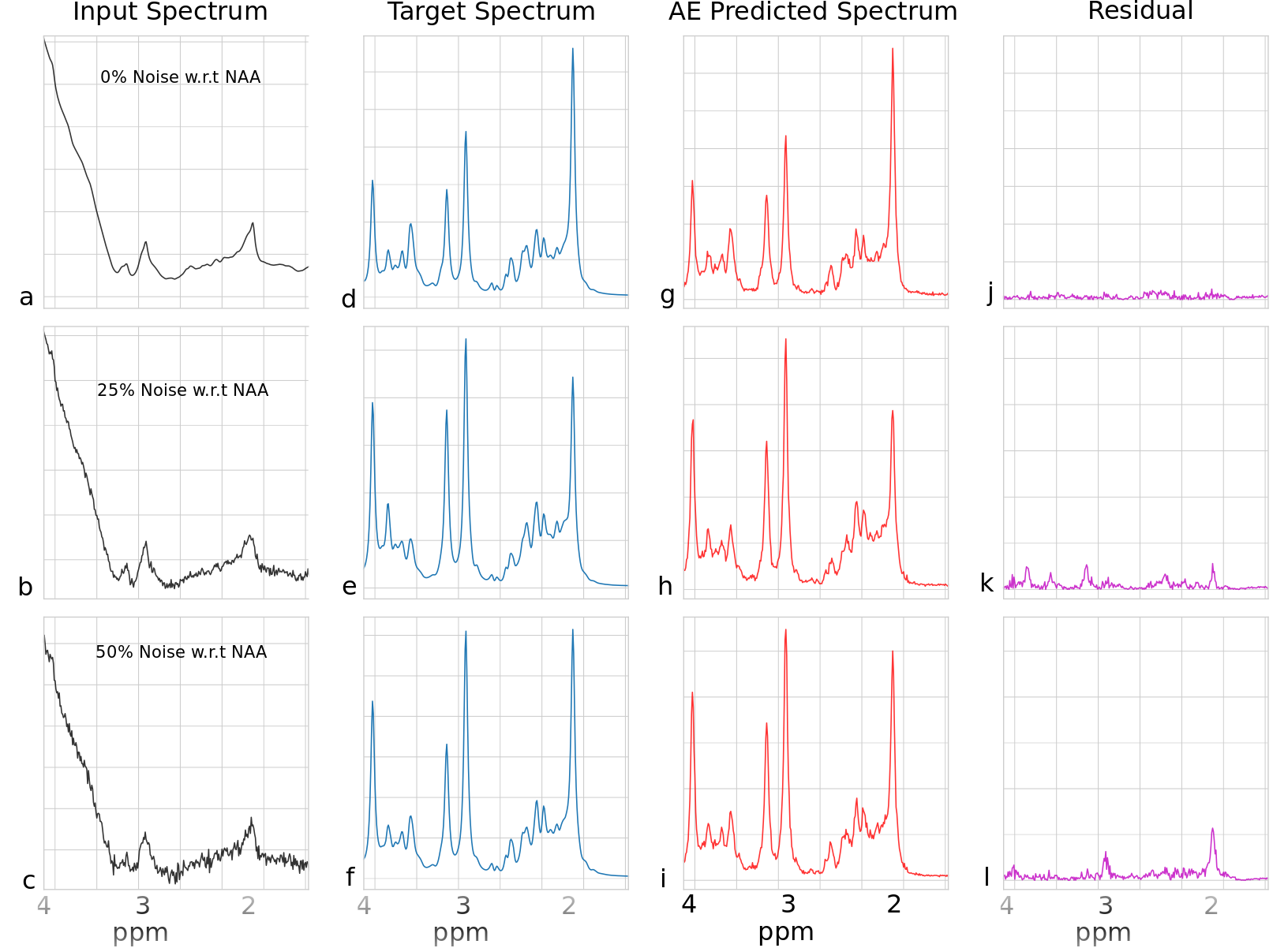
Representative simulated water unsuppressed brain spectrum and corresponding metabolite spectrum and Autoencoder(AE) predicted metabolite spectrum. a-c shows the simulated water spectrum with noise, and the water concentration is four orders of magnitude higher than metabolites, which are used inputs to the AE. d-f, target metabolite spectra, g-i shows the AE-predicted spectrum, and j-l shows the difference spectra obtained by subtracting the AE predicted spectra from the target spectra.
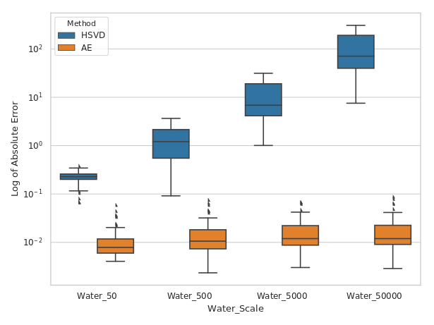
Absolute error (log scale) for water removal using Hankel Singular Value Decomposition (HSVD) and Autoencoder (AE). The absolute error for AE is computed by subtracting the AE predicted spectra from the target metabolite spectra. Similarly, for the HSVD method, the absolute error is obtained by subtracting the HSVD computed spectra from the target metabolite spectra as the water concentration is scaled up the error increases linearly for the AE method compared to HSVD method.
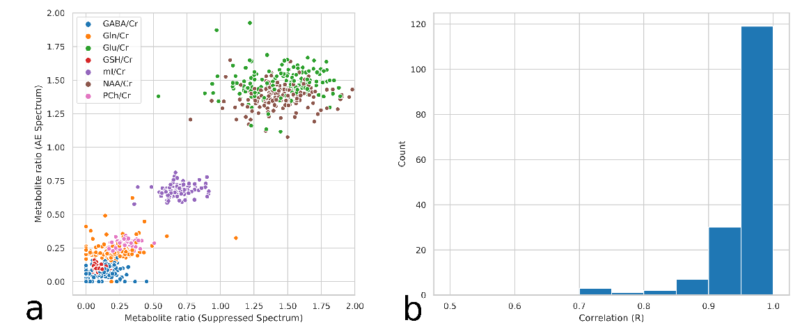
Correlation of metabolite concentration ratios obtained using LCModel, for Autoencoder (AE) predicted and water suppressed spectra for in-vivo test dataset. Comparison of the metabolite concentration ratios (a), overall, there is a strong correlation between metabolite. The clustering pattern can be caused by the reconstruction error and change in the degree of freedom of LCModel fit between the spectra. Histogram of the correlation values (b), most of the spectra have a high correlation.
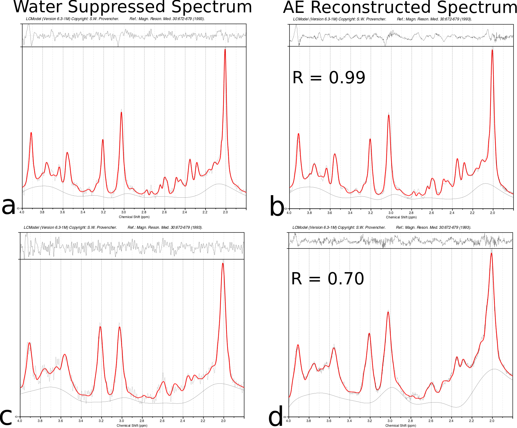
Representative water suppressed brain spectrum and Autoencoder(AE) predicted metabolite spectrum from in-vivo test dataset. The spectrum in (a) and (b) is an example of water suppressed and AE-predicted spectra with correlation R>0.9. The spectrum in (c) and (d) is an example of water suppressed and AE-predicted spectra with correlation R=0.7