1293

Gaussian Process Progression Modelling of structural MRI changes in Huntington’s disease

Peter A. Wijeratne^1,2, Sara Garbarino³, Eileanoir B. Johnson², Sarah Gregory², Rachael I. Scahill², Sarah J. Tabrizi², Marco Lorenzi³, and Daniel C. Alexander¹
¹Department of Computer Science, University College London, London, United Kingdom, ²Department of Neurodegenerative Disease, University College London, London, United Kingdom, ³Université Côte d’Azur, Valbonne, France

Synopsis

Longitudinal measurements of brain atrophy using structural T1-weighted MRI (sMRI) can provide powerful biomarkers for clinical trials in neurodegenerative diseases. Here we use the latest advances in disease progression modelling, specifically the Gaussian Process Progression Model (GPPM), to untangle the effects of inter-subject variability, measurement noise and individual disease stage on longitudinal sMRI measurements in Huntington’s disease (HD). We use GPPM to estimate, for the first time, the relative timescale of sub-cortical atrophy in HD, and identify when sMRI provides additional information to genetics. We conclude that GPPM could increase power over standard imaging biomarkers for clinical trials in HD.

Introduction

The identification of new biomarkers of disease progression is crucial for the efficient design and execution of clinical trials in Huntington’s disease (HD), and more broadly any neurodegenerative disease. Structural MRI (sMRI) can provide continuous measures that track disease progression, and can be estimated from cohort study data using methods such as voxel based morphometry [1]. However, time series analysis in medical data are confounded by inter-subject variability, measurement noise, and the lack of common reference timeline, as study participants are typically drawn from a mixture of unknown disease stages.

Disease progression modelling addresses this problem using computational methods to reconstruct long-term trajectories from short-term data [2]. We previously developed an event-based model (EBM) in HD, which estimated a sequence of sMRI changes using cross-sectional data [3]. However, EBM does not model longitudinal information which is necessary to capture variability in biomarkers for clinical trials. Here we use the recently developed Gaussian Process Progression Model (GPPM) [4] to learn a timeline common to all subjects and hence model longitudinal trajectories of regional sMRI markers in HD.

Methods

We used T1-weighted 3T sMRI scans and genetic data (number of cytosine-adenine-guanine (CAG) repeats) from 327 participants (129 healthy control; 125 pre-manifest HD; 73 manifest HD) in the TRACK-HD study [1], with a maximum of four time-points per participant. Scans were post-processed using the Geodesic Information Flows segmentation tool [5] to provide regional volume measurements. All volumes were adjusted for covariates (age, sex, site, intracranial volume).

Longitudinal change in key sMRI volumes was modelled at both the individual and group levels using the Gaussian Process Progression Model (GPPM) framework [4]. GPPM estimates a common timeline across the population, as well as a time-shift (position) for each individual along the timeline. Together this information provides a staging system, with individual stages given by the time-shift and prognosis given by the timeline.

More formally, GPPM implements time-reparameterized Gaussian Process regression [6] defined by the generative model:

$${y} ^ {j} ({ϕ} ^ {j} (t ) ) = f ({ϕ} ^ {j} (t )) + {ν} ^ {j}({ϕ} ^ {j} (t )) + ϵ ,$$
where $$${y} ^ {j}$$$ is the vector of sMRI volumes for subject j, $$${ϕ} ^ {j} (t )$$$ is the time reparameterization function, $$$f ({ϕ} ^ {j} (t ) )$$$ is the fixed-effect modelling group-wise trajectories, $$${ν} ^ {j}({ϕ} ^ {j} (t ) )$$$ is the individual random-effect, and $$$ ϵ $$$ is time-independent measurement noise. The model therefore estimates both longitudinal volumetric change at the group and individual levels, and individual time shifts along the predicted trajectory. Model parameters were estimated using the Deep Gaussian Process variational framework presented in [7] and implemented in PyTorch [8]. Individuals were assigned a time-shift according to their maximum likelihood position over all trajectories.

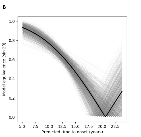
To evaluate GPPM, predicted individual-level time-shifts were compared with the predicted time-to-onset in pre-manifest participants using a benchmark non-parametric survival model based on age and CAG repeat count [9]. To determine the time window in which the two models provided equivalent information, Bayesian regression was used to fit the relationship between predicted time shifts and time-to-onset. Model equivalence was then quantified by the angle of the fit slope, θ, with maximal association (one-to-one equivalence) given at θ=$$$\pi/4$$$ and no association (orthogonality) at θ=0.

Results

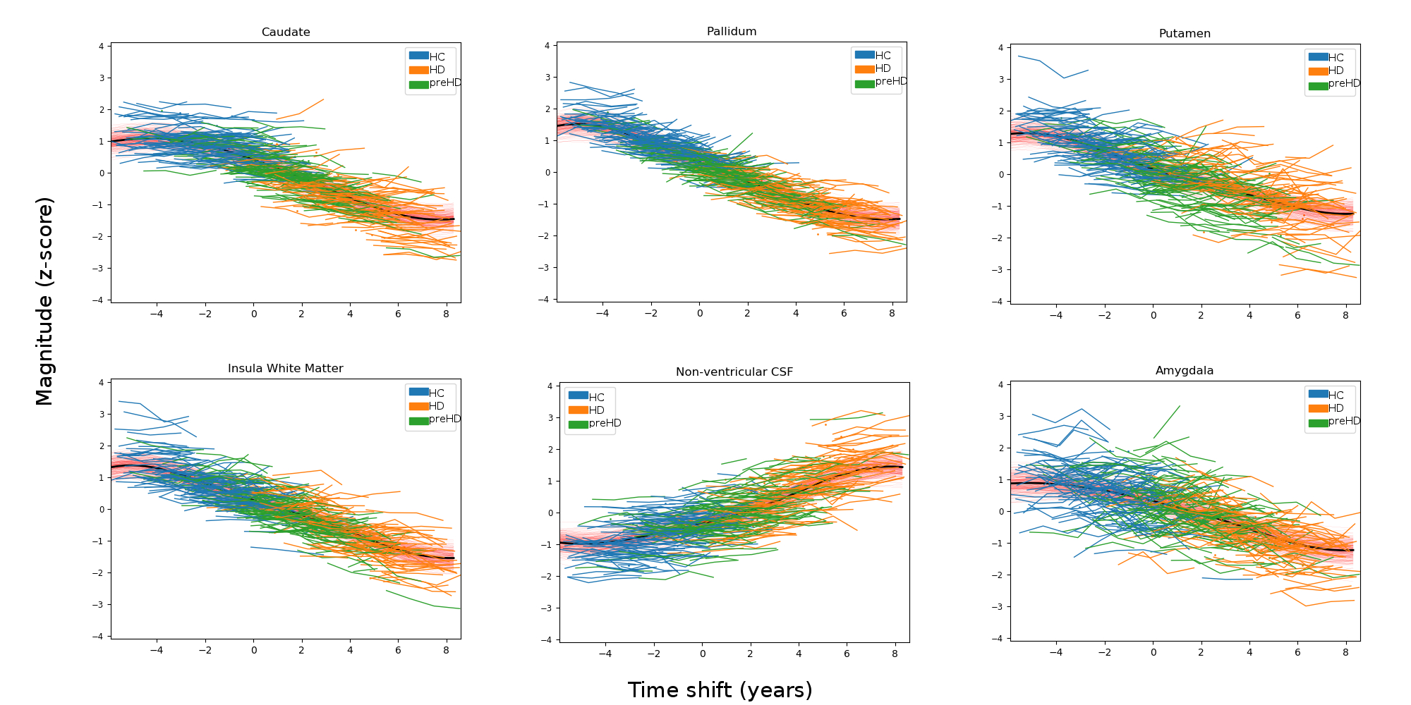
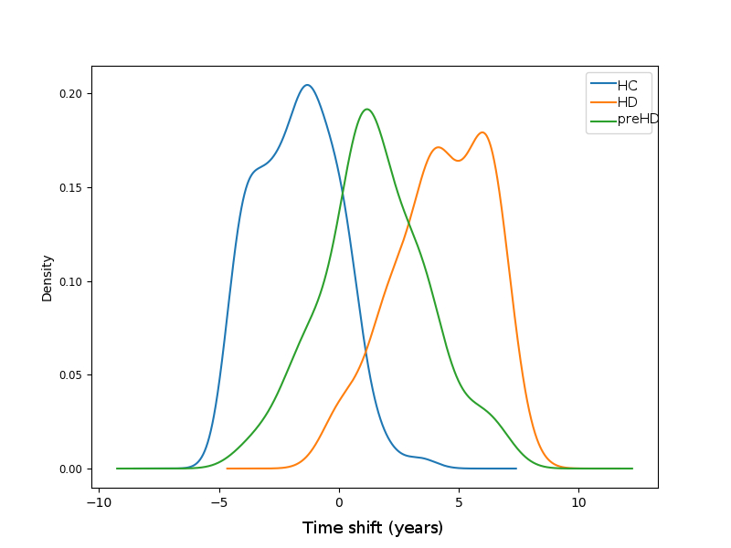
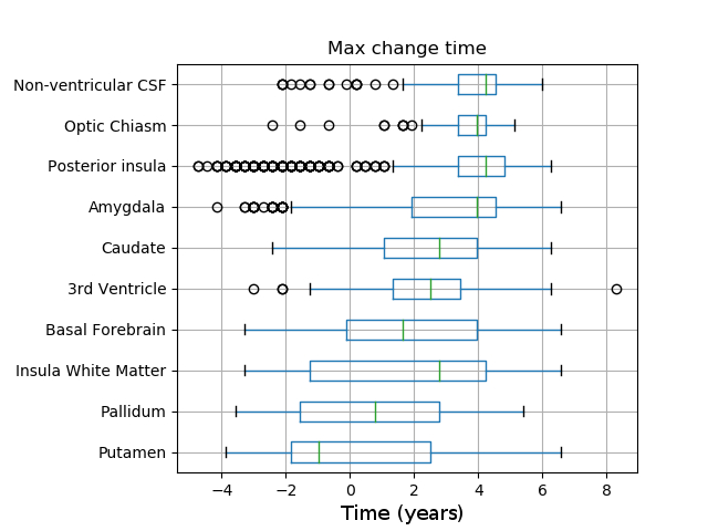
Figure 1 shows predicted volumetric trajectories in six key anatomical regions. All regions demonstrate changes in volume over time, with absolute magnitude of change ranging from 10-23% over a timeline of ~12 years. The model successfully separates the three sub-groups, with healthy controls positioned early in the trajectory, pre-manifest HD mid-way, and manifest HD at the end (Figure 2).

The model can also be used to predict the sequence of sMRI changes in time, by taking the time at maximum gradient as the time where the volume transitions from a normal to abnormal state. Figure 3 shows the maximum change time for 10 regional volumes, calculated from 1000 samples of the posterior. GPPM predicts the earliest changes in sub-cortical regions of the basal ganglia (putamen and pallidum).

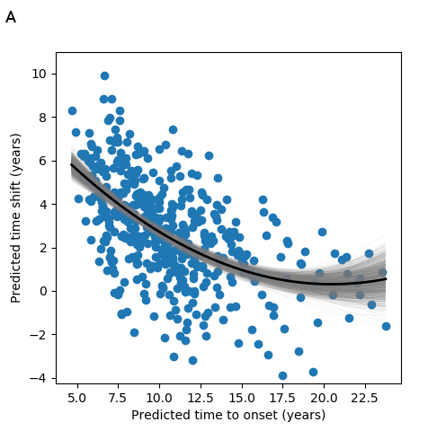
To assess the model’s predictive utility, Figure 4 shows the predicted time shift as a function of the predicted time-to-onset. We find that the timescale identified by GPPM has >0.8 equivalence to the genetic model for up to 10 years before onset, and at least 0.5 equivalence up to 15 years (Figure 5).

Discussion

GPPM recovers longitudinal changes in sMRI volumes from a large and diverse HD cohort. These regions were chosen to be the same as those from our previous analysis [3]. Interestingly, both methodologies predict the earliest changes in the putamen and pallidum, which provides strong evidence for the use of these regions as early-stage biomarkers. Unlike [3], GPPM also provides time-dependent information, which is crucial for potential biomarkers in clinical trials.

The comparison between GPPM predictions and the benchmark genetic model revealed a time window in which sMRI provides additional information to genetics. This supports the use of sMRI biomarkers with GPPMs in clinical trials in HD, as they can provide continuous measures that both reflect underlying genetic factors and track disease progression.

Conclusion

GPPM can provide new potential biomarkers for clinical trials in HD.

Acknowledgements

We thank all the participants and doctors involved in the TRACK-HD study. PAW was supported by a MRC Skills Development Fellowship (MR/T027770/1). S Garbarino was supported by L'Agence Nationale de la Recherche under Investissements d'Avenir UCA JEDI (ANR-15-IDEX-01) through the project "AtroProDem: A data-driven model of mechanistic brain Atrophy Propagation in Dementia". EBJ, S Gregory, RIS and SJT were supported by funding from the Wellcome Trust (200181/Z/15/Z). DCA was supported by funding from the European Union’s Horizon 2020 research and innovation programme under grant agreement number 666992 and from the NIHR UCLH Biomedical Research Centre. This work was supported by the Inria Sophia Antipolis - Méditerranée, "NEF" computation cluster.

References

[1] Tabrizi, S.J., Scahill R.I., Owen G., et al. Predictors of phenotypic progression and disease onset in premanifest Huntington’s disease in the TRACK-HD study: analysis of 36-month observational data. The Lance Neurology. 2013;12(7):637-649, doi:10.1016/S1474-4422(13)70088-7

[2] Oxtoby, N.P., Alexander, D.C. Imaging plus X: multimodal models of neurodegenerative disease. Curr Opin Neurol. 2017;30(4):371-379, doi:10.1097/WCO.0000000000000460

[3] Wijeratne PA, Young AL, Oxtoby NP et al. An image-based model of brain volume biomarker changes in Hungtington’s disease. Ann Clin Trans Neurol. 2018a;5(5):570-82, https://doi.org/10.1002/acn3.558

[4] Lorenzi M, Filippone M, Frisoni GB, et al. Probabilistic disease progression modeling to characterize diagnostic uncertainty: Application to staging and prediction in Alzheimer’s disease. NeuroImage. 2017;S1053-8119(17)30706-1, https://doi.org/10.1016/j.neuroimage.2017.08.059. Model available at: gpprogressionmodel.inria.fr

[5] Cardoso M.J., Modat M., Wolz R., et al. Geodesic Information Flows: Spatially-Variant Graphs and Their Application to Segmentation and Fusion. IEEE Transactions on Medical Imaging. 2015;34:1976-1988, doi: 10.1109/TMI.2015.2418298

[6] Rasmussen CE, Williams CKI. Gaussian Processes for Machine Learning. MIT Press, 2006

[7] Lorenzi, M, Filippone, M (2018). PMLR, 80:3227-3236, URL: http://proceedings.mlr.press/v80/lorenzi18a.html

[8] PyTorch: https://pytorch.org

[9] Langbehn DR, Hayden M, Paulsen JS. CAG-repeat length and the age of onset in Huntington Disease (HD): A review and validation study of statistical approaches. Am J Med Neuropsychiatr Genet. 2011;153B(2):397-408, https://doi.org/10.1002/ajmg.b.30992

Figures

Figure 1: GPPM predicted trajectories for six regional volumes. Legend – HC: healthy controls (blue); preHD: pre-manifest HD (green); HD: manifest HD (orange).

Figure 2: Time shift density for each sub-group. Legend – HC: healthy controls (blue); preHD: pre-manifest HD (green); HD: manifest HD (orange).

Figure 3: Predicted maximum change times for ten regional volumes. Box-plots represent the mean, upper and lower bounds from 1000 samples from the posterior. Extreme values are represented as black circles, while the green bars indicate the medians. Maximum change is taken to be the time at maximum gradient for each sample.

Figure 4: GPPM predicted time shift as a function of predicted time to onset. Fit is a quadratic Bayesian regression with uncertainty estimated by 1000 samples from the posterior.

Figure 5: Model equivalence as a function of predicted time to onset. The y-axis is calculate as y=sin(2θ), where θ is the angle of the regression slope in Figure 4A. Maximum model equivalence is given at sin(2θ)=1, i.e. where Predicted time shift=Predicted time to onset in Figure 4A, and no relationship is given for sin(2θ)=0.

Proc. Intl. Soc. Mag. Reson. Med. 28 (2020)

1293