1292

The substantial influence of negative sampling and prevalence when presenting classification results: case study with TOF-MRA

Tommaso Di Noto¹, Guillaume Marie¹, Sebastien Tourbier¹, Guillaume Saliou¹, Meritxell Bach Cuadra^1,2,3, Patric Hagmann¹, and Jonas Richiardi^1,4
¹Faculty of Biology and Medicine, Department of Radiology, Lausanne University Hospital (CHUV) and University of Lausanne (UNIL), Lausanne, Switzerland, ²Medical Image Analysis Laboratory (MIAL), Centre d’Imagerie BioMédicale (CIBM), Lausanne, Switzerland, ³Signal Processing Laboratory (LTS 5), Ecole Polytechnique Fédérale de Lausanne (EPFL), Lausanne, Switzerland, ⁴Advanced Clinical Imaging Technology, Siemens Healthcare, Lausanne, Switzerland

Synopsis

One recurrent problem for applying deep learning models in medical imaging is the reduced availability of labelled training data. A common approach is therefore to focus on image patches rather than whole volumes, thus increasing the number of samples. However, for many diseases anomalous patches (positive samples) are outnumbered by negative patches showing no anomaly. Here, we explore different strategies for negative sampling in the context of brain aneurysm detection. We show that classification performances can vary drastically with respect to negative sampling, and that real-world disease or anomaly prevalence can further degrade performance estimates.

Introduction

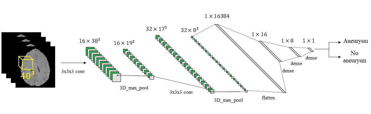
Magnetic Resonance Angiography (MRA) is routinely performed to monitor/detect intracranial aneurysms. From MRA volumes, most recent studies^1-4 then usually carry out tasks such as segmentation or classification (detection). In the past few years, both of these tasks have been drastically changed due to progress in deep learning (DL) algorithms⁵. However, along with the benefits brought by DL, several challenges also became evident, such as the limited availability of training examples for building models that do not suffer from overfitting⁶. A common practice adopted to mitigate this problem consists in analyzing 3D patches extracted from the available patient scans, instead of the entire volumes, to increase the dataset dimension^7-14. While for the minority class (e.g. anomaly of interest, such as an aneurysm/lesion) this operation is restricted by the availability of positive cases, extraction of negative samples (majority-class negative sampling) comes with a challenge: the choice of the extraction criterion. Narrowing just to classification, indeed extracted negative patches could be too easily classified by the model, due for instance to gross intensity or anatomical differences. This choice can dramatically alter final results, along with the oftentimes-forgotten real-world prevalence adjustment for the study population. Though similar works^2,15 mentioned the potential effect of prevalence, none of them corrected classification metrics accordingly. In this regard, this work explores how classification performances of a convolutional neural network (CNN) used to detect brain aneurysms in Time-of-Flight MRA (TOF-MRA) can vary with respect to the negative sampling strategy used and to different levels of disease/anomaly prevalence.

Methods

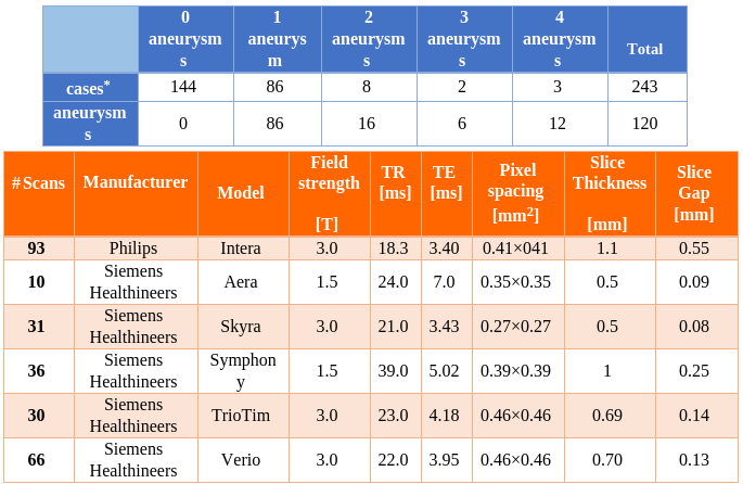
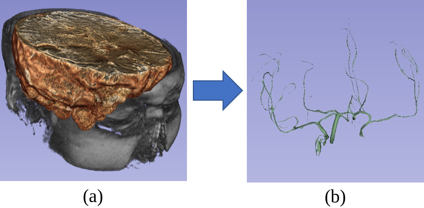
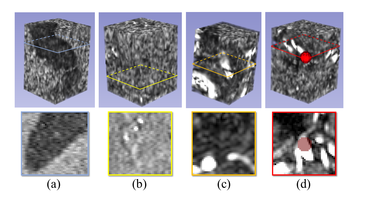
A retrospective cohort of 232 subjects who underwent clinically-indicated TOF-MRA between 2010 and 2012 was used. Patients with one or more unruptured intracranial aneurysms were included, while treated and ruptured aneurysms were excluded. Out of 232, 88 had one (or more) aneurysm(s), while 144 did not present any. The overall number of aneurysms is 120. A 3D gradient recalled echo sequence with Partial Fourier technique was used for all subjects. Figure 1 illustrates details about the population and the MR acquisition. Manual masks were drawn around aneurysms by one reader with 3 years of experience in neuroimaging and were used to distinguish positive/negative patches. Different aneurysms of the same patient were treated as independent. Similarly, for patients with multiple sessions, we treated each session independently. The dataset was organized according to the Brain Imaging Data Structure (BIDS)¹⁶ standard. Data was pre-processed as illustrated in Figure 2. First, we performed brain extraction with the Brain Extraction Tool¹⁷. Second, the Vascular Modelling Toolkit¹⁸ was used to extract a vessel mask of each subject. After preprocessing, three datasets (henceforth D1, D2, D3) were created. While positive patches were centered around the aneurysms and identical for the three datasets, the following strategies were applied for negative sampling (all without overlap with aneurysms), in increasing order of difficulty for the network:

For D1, negative patches were extracted randomly within the pre-processed brain.
For D2, we imposed an intensity threshold for the extraction: with an iterative search we only extracted the patch when its average brightness was higher than a threshold which, in turn, was chosen according to the average brightness of positive patches. This avoids extracting patches that are too dark with respect to positive ones which include vessels and therefore are usually brighter.
The iterative search for D3 only extracted the negative patch if the percentage of vessel voxels (obtained with VMTK masks) was higher than a certain threshold within the candidate volume. This was performed to ensure that also patches containing vessels without aneurysms were included. Again, the threshold was chosen according to the average percentage of vessel voxels found in positive patches.

For all datasets, we extracted 741 negative and 120 positive patches. Each dataset was split into training (70%), validation (15%) and test (15%) set to fit the model, tune its hyperparameters and report final results, respectively. Three negative patches taken from D1, D2 and D3, plus one positive patch are shown in Figure 3, while the structure of the network is illustrated in Figure 4. When presenting classification results, along with standard metrics, we included two additional ones, namely real-world PPV and real-world NPV as ¹⁹. These are computed specifying an explicit prevalence: $$RW\_PPV = \frac{Sensitivity*Prevalence}{Sensitivity*Prevalence+(1-Specificity)*(1-Prevalence)}$$ $$RW\_NPV = \frac{Specificity*(1-Prevalence)}{Specificity*(1-Prevalence)+(1-Sensitivity)*Prevalence}$$ Here, we corrected PPV and NPV with a 5% prevalence (i.e. aneurysm prevalence in TOF-MRA patients²⁰).

Results

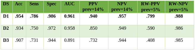
Figure 5 shows classification results achieved by our CNN on the untouched test sets. When taking true prevalence into account (RW-PPV), results decrease dramatically for D2 and D3, whereas they remain acceptable for D1. Moreover, as expected, performances decrease as negative sampling difficulty increases.

Discussion

This work demonstrates how classification results that at first glance might seem promising, should instead always be contextualized with respect to the disease prevalence and to the negative sampling technique. Indeed, seemingly small differences between good results can be magnified dramatically when real-world prevalence is considered. Furthermore, the choice of the negative sampling strategy must also be clearly specified since it can likewise alter results significantly. In clinical setting, where the whole brain would be scanned patch-wise for aneurysm detection, we expect performances to be lower-bounded by D3 and upper-bounded by D1.

Acknowledgements

No acknowledgement found.

References

1. Ueda, D., Yamamoto, A., Nishimori, M., Shimono, T., Doishita, S., Shimazaki, A., ... & Miki, Y. (2018). Deep learning for MR angiography: automated detection of cerebral aneurysms. Radiology, 290(1), 187-194.

2. Sichtermann, T., Faron, A., Sijben, R., Teichert, N., Freiherr, J., & Wiesmann, M. (2019). Deep Learning–Based Detection of Intracranial Aneurysms in 3D TOF-MRA. American Journal of Neuroradiology, 40(1), 25-32.

3. Nakao, T., Hanaoka, S., Nomura, Y., Sato, I., Nemoto, M., Miki, S., ... & Abe, O. (2018). Deep neural network‐based computer‐assisted detection of cerebral aneurysms in MR angiography. Journal of Magnetic Resonance Imaging, 47(4), 948-953.

4. Stember, J. N., Chang, P., Stember, D. M., Liu, M., Grinband, J., Filippi, C. G., ... & Jambawalikar, S. (2019). Convolutional neural networks for the detection and measurement of cerebral aneurysms on magnetic resonance angiography. Journal of digital imaging, 32(5), 808-815.

5. Syeda-Mahmood, T. (2018). Role of big data and machine learning in diagnostic decision support in radiology. Journal of the American College of Radiology, 15(3), 569-576.

6. Shen, D., Wu, G., & Suk, H. I. (2017). Deep learning in medical image analysis. Annual review of biomedical engineering, 19, 221-248.

7. Suk, H. I., Lee, S. W., Shen, D., & Alzheimer's Disease Neuroimaging Initiative. (2014). Hierarchical feature representation and multimodal fusion with deep learning for AD/MCI diagnosis. NeuroImage, 101, 569-582.

8. Cheng, J. Z., Ni, D., Chou, Y. H., Qin, J., Tiu, C. M., Chang, Y. C., ... & Chen, C. M. (2016). Computer-aided diagnosis with deep learning architecture: applications to breast lesions in US images and pulmonary nodules in CT scans. Scientific reports, 6, 24454.

9. Roth, H. R., Lu, L., Liu, J., Yao, J., Seff, A., Cherry, K., ... & Summers, R. M. (2015). Improving computer-aided detection using convolutional neural networks and random view aggregation. IEEE transactions on medical imaging, 35(5), 1170-1181.

10. Shen, W., Zhou, M., Yang, F., Yang, C., & Tian, J. (2015, June). Multi-scale convolutional neural networks for lung nodule classification. In International Conference on Information Processing in Medical Imaging (pp. 588-599). Springer, Cham.

11. Setio, A. A. A., Ciompi, F., Litjens, G., Gerke, P., Jacobs, C., Van Riel, S. J., ... & van Ginneken, B. (2016). Pulmonary nodule detection in CT images: false positive reduction using multi-view convolutional networks. IEEE transactions on medical imaging, 35(5), 1160-1169.

12. Ciompi, F., de Hoop, B., van Riel, S. J., Chung, K., Scholten, E. T., Oudkerk, M., ... & van Ginneken, B. (2015). Automatic classification of pulmonary peri-fissural nodules in computed tomography using an ensemble of 2D views and a convolutional neural network out-of-the-box. Medical image analysis, 26(1), 195-202.

13. Li, R., Zhang, W., Suk, H. I., Wang, L., Li, J., Shen, D., & Ji, S. (2014, September). Deep learning based imaging data completion for improved brain disease diagnosis. In International Conference on Medical Image Computing and Computer-Assisted Intervention (pp. 305-312). Springer, Cham.

14. Shin, H. C., Roth, H. R., Gao, M., Lu, L., Xu, Z., Nogues, I., ... & Summers, R. M. (2016). Deep convolutional neural networks for computer-aided detection: CNN architectures, dataset characteristics and transfer learning. IEEE transactions on medical imaging, 35(5), 1285-1298.

15. Park, A., Chute, C., Rajpurkar, P., Lou, J., Ball, R. L., Shpanskaya, K., ... & Ni, J. (2019). Deep Learning–Assisted Diagnosis of Cerebral Aneurysms Using the HeadXNet Model. JAMA network open, 2(6), e195600-e195600.

16. Gorgolewski, K. J., Auer, T., Calhoun, V. D., Craddock, R. C., Das, S., Duff, E. P., ... & Handwerker, D. A. (2016). The brain imaging data structure, a format for organizing and describing outputs of neuroimaging experiments. Scientific Data, 3, 160044.

17. Smith, S. M. (2002). Fast robust automated brain extraction. Human brain mapping, 17(3), 143-155.

18. Piccinelli, M., Veneziani, A., Steinman, D. A., Remuzzi, A., & Antiga, L. (2009). A framework for geometric analysis of vascular structures: application to cerebral aneurysms. IEEE transactions on medical imaging, 28(8), 1141-1155.

19. Castellanos, F. X., Di Martino, A., Craddock, R. C., Mehta, A. D., & Milham, M. P. (2013). Clinical applications of the functional connectome. Neuroimage, 80, 527-540.

20. Jeon, T. Y., Jeon, P., & Kim, K. H. (2011). Prevalence of unruptured intracranial aneurysm on MR angiography. Korean journal of radiology, 12(5), 547-553.

Figures

Upper table: distribution of patients and corresponding aneurysms. *Each session was treated as a distinct case; hence, we finally extract patches from 243 cases, even though our cohort is made of 232 subjects. Lower table: MR acquisition parameters of the study population.

(a): Example of one TOF-MRA scan and corresponding brain extraction (brown) performed with Brain Extraction Tool - BET. (b): Brain vessel mask computed with Vascular Modelling Toolkit – VMTK from the skull-stripped volume.

One negative patch and a corresponding axial slice extracted from (a) D1 (random sampling), (b) D2 (intensity-matched sampling) and (c) D3 (vesselness-matched sampling), respectively. (d) Positive patch and one axial slice, along with the red annotation of one aneurysm. All patches have size 40^3.

3D-Convolutional Neural Network used to classify MRA patches. The final output is either positive (patch with aneurysm) or negative (no aneurysm). Each layer has ReLU activation function, except the last dense layer which has a sigmoid function. Adam optimizer was used. Learning rate (LR), #epochs (E), batch size (BS), dropout rate (DR), #conv layers and #dense nodes were tuned with the validation set. This led to the following hyperparameters for test evaluation: LR=1e-05, BS=32, E=25, DR=0.

Classification results for D1, D2 and D3. For each dataset, a separate untouched test set was created and used for computing the results. DS = data set, Acc = accuracy, Sens = sensitivity, Spec = specificity, AUC = Area Under ROC Curve, RW-PPV = real-world positive predictive value, RW-NPV = real-world negative predictive value. The 14% prevalence value comes from the two classes distribution in D1, D2 and D3. Boldface numbers represent highest results.

Proc. Intl. Soc. Mag. Reson. Med. 28 (2020)

1292